Critical Assessment of Metagenome Interpretation—a benchmark of metagenomics software (original) (raw)

Main

The biological interpretation of metagenomes relies on sophisticated computational analyses such as read assembly, binning and taxonomic profiling. Tremendous progress has been achieved1, but there is still much room for improvement. The evaluation of computational methods has been limited largely to publications presenting novel or improved tools. These results are extremely difficult to compare owing to varying evaluation strategies, benchmark data sets and performance criteria. Furthermore, the state of the art in this active field is a moving target, and the assessment of new algorithms by individual researchers consumes substantial time and computational resources and may introduce unintended biases.

We tackle these challenges with a community-driven initiative for the Critical Assessment of Metagenome Interpretation (CAMI). CAMI aims to evaluate methods for metagenome analysis comprehensively and objectively by establishing standards through community involvement in the design of benchmark data sets, evaluation procedures, choice of performance metrics and questions to focus on. To generate a comprehensive overview, we organized a benchmarking challenge on data sets of unprecedented complexity and degree of realism. Although benchmarking has been performed before2,3, this is the first community-driven effort that we know of. The CAMI portal is also open to submissions, and the benchmarks generated here can be used to assess and develop future work.

We assessed the performance of metagenome assembly, binning and taxonomic profiling programs when encountering major challenges commonly observed in metagenomics. For instance, microbiome research benefits from the recovery of genomes for individual strains from metagenomes4,5,6,7, and many ecosystems have a high degree of strain heterogeneity8,9. To date, it is not clear how much assembly, binning and profiling software are influenced by the evolutionary relatedness of organisms, community complexity, presence of poorly categorized taxonomic groups (such as viruses) or varying software parameters.

Results

We generated extensive metagenome benchmark data sets from newly sequenced genomes of ∼700 microbial isolates and 600 circular elements that were distinct from strains, species, genera or orders represented by public genomes during the challenge. The data sets mimicked commonly used experimental settings and properties of real data sets, such as the presence of multiple, closely related strains, plasmid and viral sequences and realistic abundance profiles. For reproducibility, CAMI challenge participants were encouraged to provide predictions along with an executable Docker biobox10 implementing their software and specifying the parameter settings and reference databases used. Overall, 215 submissions, representing 25 programs and 36 biobox implementations, were received from 16 teams worldwide, with consent to publish (Online Methods).

Assembly challenge

Assembling genomes from metagenomic short-read data is very challenging owing to the complexity and diversity of microbial communities and the fact that closely related genomes may represent genome-sized approximate repeats. Nevertheless, sequence assembly is a crucial part of metagenome analysis, and subsequent analyses—such as binning—depend on the assembly quality.

Overall performance trends

Developers submitted reproducible results for six assemblers: MEGAHIT11, Minia12, Meraga (Meraculous13 + MEGAHIT), A* (using the OperaMS Scaffolder)14, Ray Meta15 and Velour16. Several are dedicated metagenome assemblers, while others are more broadly used (Supplementary Tables 1 and 2). Across all data sets (Supplementary Table 3) the assembly statistics (Online Methods) varied substantially by program and parameter settings (Supplementary Figs. 1–12). The gold-standard co-assembly of the five samples constituting the high-complexity data set has 2.80 Gbp in 39,140 contigs. The assembly results ranged from 12.32 Mbp to 1.97 Gbp in size (0.4% and 70% of the gold standard co-assembly, respectively), 0.4% to 69.4% genome fraction, 11 to 8,831 misassemblies and 249 bp to 40.1 Mbp unaligned contigs (Supplementary Table 4 and Supplementary Fig. 1). MEGAHIT11 produced the largest assembly, of 1.97 Gbp, with 587,607 contigs, 69.3% genome fraction and 96.9% mapped reads. It had a substantial number of unaligned bases (2.28 Mbp) and the most misassemblies (8,831). Changing the parameters of MEGAHIT (Megahit_ep_mtl200) substantially increased the unaligned bases, to 40.89 Mbp, whereas the total assembly length, genome fraction and fraction of mapped reads remained almost identical (1.94 Gbp, 67.3% and 97.0%, respectively, with 7,538 misassemblies). Minia12 generated the second largest assembly (1.85 Gbp in 574,094 contigs), with a genome fraction of 65.7%, only 0.12 Mbp of unaligned bases and 1,555 misassemblies. Of all reads, 88.1% mapped to the Minia assembly. Meraga generated an assembly of 1.81 Gbp in 745,109 contigs, to which 90.5% of reads mapped (2.6 Mbp unaligned, 64.0% genome fraction and 2,334 misassemblies). Velour (VELOUR_k63_C2.0) produced the most contigs (842,405) in a 1.1-Gbp assembly (15.0% genome fraction), with 381 misassemblies and 56 kbp unaligned sequences. 81% of the reads mapped to the Velour assembly. The smallest assembly was produced by Ray6 using _k_-mer of 91 (Ray_k91) with 12.3 Mbp assembled into 13,847 contigs (genome fraction <0.1%). Only 3.2% of the reads mapped to this assembly.

Altogether, MEGAHIT, Minia and Meraga produced results of similar quality when considering these various metrics; they generated a higher contiguity than the other assemblers (Supplementary Figs. 10–12) and assembled a substantial fraction of genomes across a broad abundance range. Analysis of the low- and medium-complexity data sets delivered similar results (Supplementary Figs. 4–9).

Closely related genomes

To assess how the presence of closely related genomes affects assemblies, we divided genomes according to their average nucleotide identity (ANI)17 into 'unique strains' (genomes with <95% ANI to any other genome) and 'common strains' (genomes with an ANI ≥95% to another genome in the data set). Meraga, MEGAHIT and Minia recovered the largest fraction of all genomes (Fig. 1a). For unique strains, Minia and MEGAHIT recovered the highest percentages (median over all genomes 98.2%), followed by Meraga (median 96%) and _VELOUR_k31_C2.0_ (median 62.9%) (Fig. 1b). Notably, for the common strains, all assemblers recovered a substantially lower fraction (Fig. 1c). MEGAHIT (_Megahit_ep_mtl200_; median 22.5%) was followed by Meraga (median 12.0%) and Minia (median 11.6%), whereas _VELOUR_k31_C2.0_ recovered only 4.1% (median). Thus, the metagenome assemblers produced high-quality results for genomes without close relatives, while only a small fraction of the common strain genomes was assembled, with assembler-specific differences. For very high ANI groups (>99.9%), most assemblers recovered single genomes (Supplementary Fig. 13). Resolving strain-level diversity posed a substantial challenge to all programs evaluated.

Figure 1: Assembly results for the CAMI high-complexity data set.

(a–c) Fractions of reference genomes assembled by each assembler for all genomes (a), genomes with ANI < 95% (b) and genomes with ANI ≥95% (c). Colors indicate results from the same assembler incorporated in different pipelines or parameter settings (see Supplementary Table 2 for details). Dots indicate individual data points (genomes); boxes, interquartile range; center lines, median. (d) Genome recovery fraction versus genome sequencing depth (coverage). Data were classified as unique genomes (ANI <95%, brown), genomes with related strains present (ANI ≥95%, blue) or high-copy circular elements (green). The gold standard includes all genomic regions covered by at least one read in the metagenome data set.

Source data

Full size image

Effect of sequencing depth

To investigate the effect of sequencing depth on the assemblies, we compared the genome recovery rate (genome fraction) to the genome sequencing coverage (Fig. 1d and Supplementary Fig. 2 for complete results). Assemblers using multiple _k_-mers (Minia, MEGAHIT and Meraga) substantially outperformed single _k_-mer assemblers. The chosen _k_-mer size affects the recovery rate (Supplementary Fig. 3): while small _k_-mers improved recovery of low-abundance genomes, large _k_-mers led to a better recovery of highly abundant ones. Most assemblers except for Meraga and Minia did not recover very-high-copy circular elements (sequencing coverage >100×) well, though Minia lost all genomes with 80–200× sequencing coverage (Fig. 1d). Notably, no program investigated contig topology to determine whether these were circular and complete.

Binning challenge

Metagenome assembly programs return mixtures of variable-length fragments originating from individual genomes. Binning algorithms were devised to classify or bin these fragments—contigs or reads—according to their genomic or taxonomic origins, ideally generating draft genomes (or pan-genomes) of a strain (or higher-ranking taxon) from a microbial community. While genome binners group sequences into unlabeled bins, taxonomic binners group the sequences into bins with a taxonomic label attached.

Results were submitted together with software bioboxes for five genome binners and four taxonomic binners: MyCC18, MaxBin 2.0 (ref. 19), MetaBAT20, MetaWatt 3.5 (ref. 21), CONCOCT22, PhyloPythiaS+23, taxator-tk24, MEGAN6 (ref. 25) and Kraken26. Submitters ran their programs on the gold-standard co-assemblies or on individual read samples (MEGAN6), according to their suggested application. We determined their performance for addressing important questions in microbiome studies.

Recovery of individual genome bins

We investigated program performance when recovering individual genome (strain-level) bins (Online Methods). For the genome binners, average genome completeness (34% to 80%) and purity (70% to 97%) varied substantially (Supplementary Table 5 and Supplementary Fig. 14). For the medium- and low-complexity data sets, MaxBin 2.0 had the highest values (70–80% completeness, >92% purity), followed by other programs with comparably good performance in a narrow range (completeness ranging with one exception from 50–64%, >75% purity). Notably, other programs assigned a larger portion of the data sets than MaxBin 2.0 measured in bp, though with lower adjusted Rand index (ARI; Fig. 2a). For applications where binning a larger fraction of the data set at the cost of some accuracy is important, MetaWatt 3.5, MetaBAT and CONCOCT could be good choices. The high-complexity data set was more challenging to all programs, with average completeness decreasing to ∼50% and more than 70% purity, except for MaxBin 2.0 and MetaWatt 3.5, which showed purity of above 90%. The programs either assigned only a smaller data set portion (>50%, in the case of MaxBin 2.0) with high ARI or a larger fraction with lower ARI (more than 90% with less than 0.5 ARI, all except MaxBin and MetaBat). The exception was MetaWatt 3.5, which assigned more than 90% of the data set with an ARI larger than 0.8, thus best recovering abundant genomes from the high-complexity data set. Accordingly, MetaWatt 3.5, followed by MaxBin 2.0, recovered the most genomes with high purity and completeness from all data sets (Fig. 2b).

Figure 2: Binning results for the CAMI data sets.

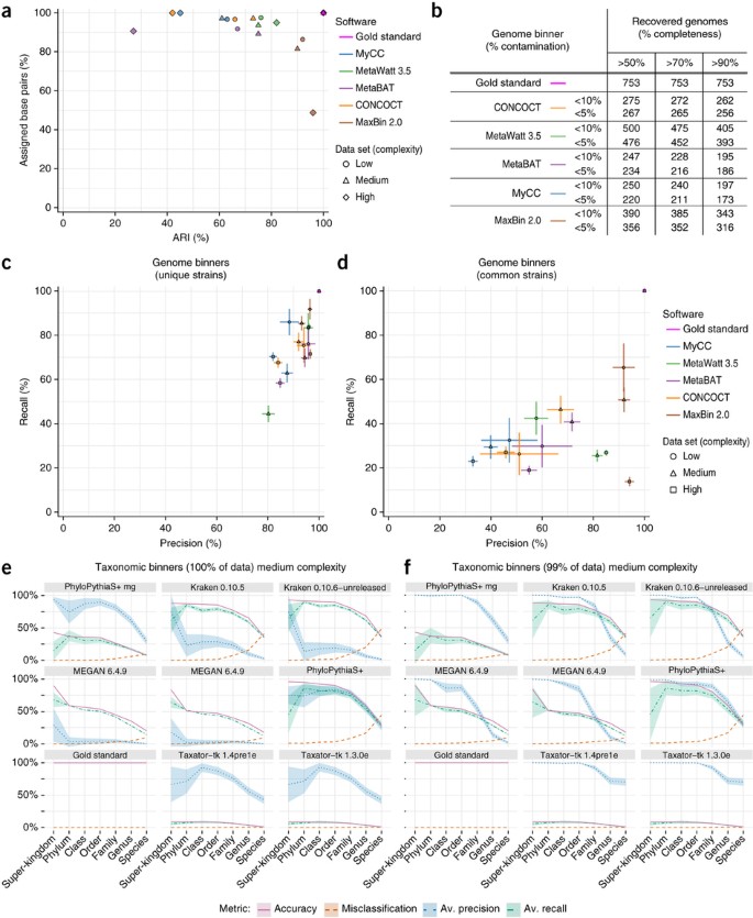
(a) ARI in relation to the fraction of the sample assigned (in bp) by the genome binners. The ARI was calculated excluding unassigned sequences and thus reflects the assignment accuracy for the portion of the data assigned. (b) Number of genomes recovered with varying completeness and contamination (1-purity). (c,d) Average purity (precision) and completeness (recall) for genomes reconstructed by genome binners for genomes of unique strains with ANI <95% to others (c) and common strains with ANI ≥95% to each other (d). For each program and complexity data set (Supplementary Table 2), the submission with the largest sum of purity and completeness is shown. In each case, small bins adding up to 1% of the data set size were removed. Error bars, s.e.m. (e,f) Taxonomic binning performance metrics across ranks for the medium-complexity data set, with results for the complete data set (e) and smallest predicted bins summing up to 1% of the data set (f) removed. Shaded areas, s.e.m. in precision (purity) and recall (completeness) across taxon bins.

Source data

Full size image

Effect of strain diversity

For unique strains, the average purity and completeness per genome bin was higher for all genome binners (Fig. 2c). For the medium- and low-complexity data sets, all had a purity of above 80%, while completeness was more variable. MaxBin 2.0 performed best across all data sets, with more than 90% purity and completeness of 70% or higher. MetaBAT, CONCOCT and MetaWatt 3.5 performed almost as well for two data sets.

For the common strains, however, completeness decreased substantially (Fig. 2d), similarly to purity for most programs. MaxBin 2.0 still stood out, with more than 90% purity on all data sets. Notably, when we considered the value of taxon bins for genome reconstruction, taxon bins had lower completeness but reached a similar purity, thus delivering high-quality, partial genome bins (Supplementary Note 1 and Supplementary Fig. 15). Overall, very high-quality genome bins were reconstructed with genome binning programs for unique strains, whereas the presence of closely related strains presented a notable hurdle.

Performance in taxonomic binning

We next investigated the performance of taxonomic binners in recovering taxon bins at different ranks (Online Methods). These results can be used for taxon-level evolutionary or functional pan-genome analyses and conversion into taxonomic profiles.

For the low-complexity data set, PhyloPythiaS+ had the highest sample assignment accuracy, average taxon bin completeness and purity, which were all above 75% from domain to family level. Kraken followed, with average completeness and accuracy still above 50% to the family level. However, purity was notably lower, owing mainly to prediction of many small false bins, which affects purity more than overall accuracy (Supplementary Fig. 16). Removing the smallest predicted bins (1% of the data set) increased purity for Kraken, MEGAN and, most strongly, for taxator-tk, for which it was close to 100% until order level, and above 75% until family level (Supplementary Fig. 17). Thus, small bins predicted by these programs are not reliable, but otherwise, high purity can be reached for higher ranks. Below the family level, all programs performed poorly, either assigning very little data (low completeness and accuracy, accompanied by a low misclassification rate) or assigning more, with substantial misclassification. Notably, Kraken and MEGAN performed similarly. These programs utilize different data properties (Supplementary Table 1) but rely on similar algorithms.

The results for the medium-complexity data set agreed qualitatively with those for the low-complexity data set, except that Kraken, MEGAN and taxator-tk performed better (Fig. 2e). With the smallest predicted bins removed, both Kraken and PhyloPythiaS+ reached above 75% for accuracy, with average completeness and purity until family rank (Fig. 2f). Similarly, taxator-tk showed an average purity of almost 75% even at genus level (almost 100% until order level), and MEGAN showed an average purity of more than 75% at order level while maintaining accuracy and average completeness of around 50%. The results of high-purity taxonomic predictions can be combined with genome bins to enable their taxonomic labeling. The performances on the high-complexity data set were similar (Supplementary Figs. 18 and 19).

Analysis of low-abundance taxa

We determined which programs delivered high completeness for low-abundance taxa. This is relevant when screening for pathogens in diagnostic settings27 or for metagenome studies of ancient DNA samples. Even though PhyloPythiaS+ and Kraken had high completeness until family rank (Fig. 2e,f), completeness degraded at lower ranks and for low-abundance bins (Supplementary Fig. 20), which are most relevant for these applications. It therefore remains a challenge to further improve predictive performance.

Deep branchers

Taxonomic binners commonly rely on comparisons to reference sequences for taxonomic assignment. To investigate the effect of increasing evolutionary distances between a query sequence and available genomes, we partitioned the challenge data sets by their taxonomic distances to public genomes as genomes of new strains, species, genus or family (Supplementary Fig. 21). For new strain genomes from sequenced species, all programs performed well, with generally high purity and, often, high completeness, or with characteristics also observed for other data sets (such as low completeness for taxator-tk). At increasing taxonomic distances to the reference, both purity and completeness for MEGAN and Kraken dropped substantially, while PhyloPythiaS+ decreased most notably in purity, and taxator-tk, in completeness. For genomes at larger taxonomic distances ('deep branchers'), PhyloPythiaS+ maintained the best purity and completeness.

Influence of plasmids and viruses

The presence of plasmid and viral sequences had almost no effect on binning performance. Although the copy numbers were high, in terms of sequence size, the fraction was small (<1.5%, Supplementary Table 6). Only Kraken and MEGAN made predictions for the viral fraction of the data or predicted viruses to be present, albeit with low purity (<30%) and completeness (<20%).

Profiling challenge

Taxonomic profilers predict the taxonomic identities and relative abundances of microbial community members from metagenome samples and are used to study the composition, diversity and dynamics of microbial communities in a variety of environments28,29,30. In contrast to taxonomic binning, profiling does not assign individual sequences. In some use cases, such as identification of potentially pathogenic organisms, accurate determination of the presence or absence of a particular taxon is important. In comparative studies (such as quantifying the dynamics of a microbial community over an ecological gradient), accurately determining the relative abundance of organisms is paramount.

Challenge participants submitted results for ten profilers: CLARK31; Common Kmers (an early version of MetaPalette)32; DUDes33; FOCUS34; MetaPhlAn 2.0 (ref. 35); MetaPhyler36; mOTU37; a combination of Quikr38, ARK39 and SEK40 (abbreviated Quikr); Taxy-Pro41 and TIPP42. Some programs were submitted with multiple versions or different parameter settings, bringing the number of unique submissions to 20.

Performance trends

We employed commonly used metrics (Online Methods) to assess the quality of taxonomic profiling submissions with regard to the biological questions outlined above. The reconstruction fidelity for all profilers varied markedly across metrics, taxonomic ranks and samples. Each had a unique error profile and different strengths and weaknesses (Fig. 3a,b), but the profilers fell into three categories: (i) profilers that correctly predicted relative abundances, (ii) precise profilers and (iii) profilers with high recall. We quantified this with a global performance summary score (Online Methods, Fig. 3c, Supplementary Figs. 22–28 and Supplementary Table 7).

Figure 3: Profiling results for the CAMI data sets.

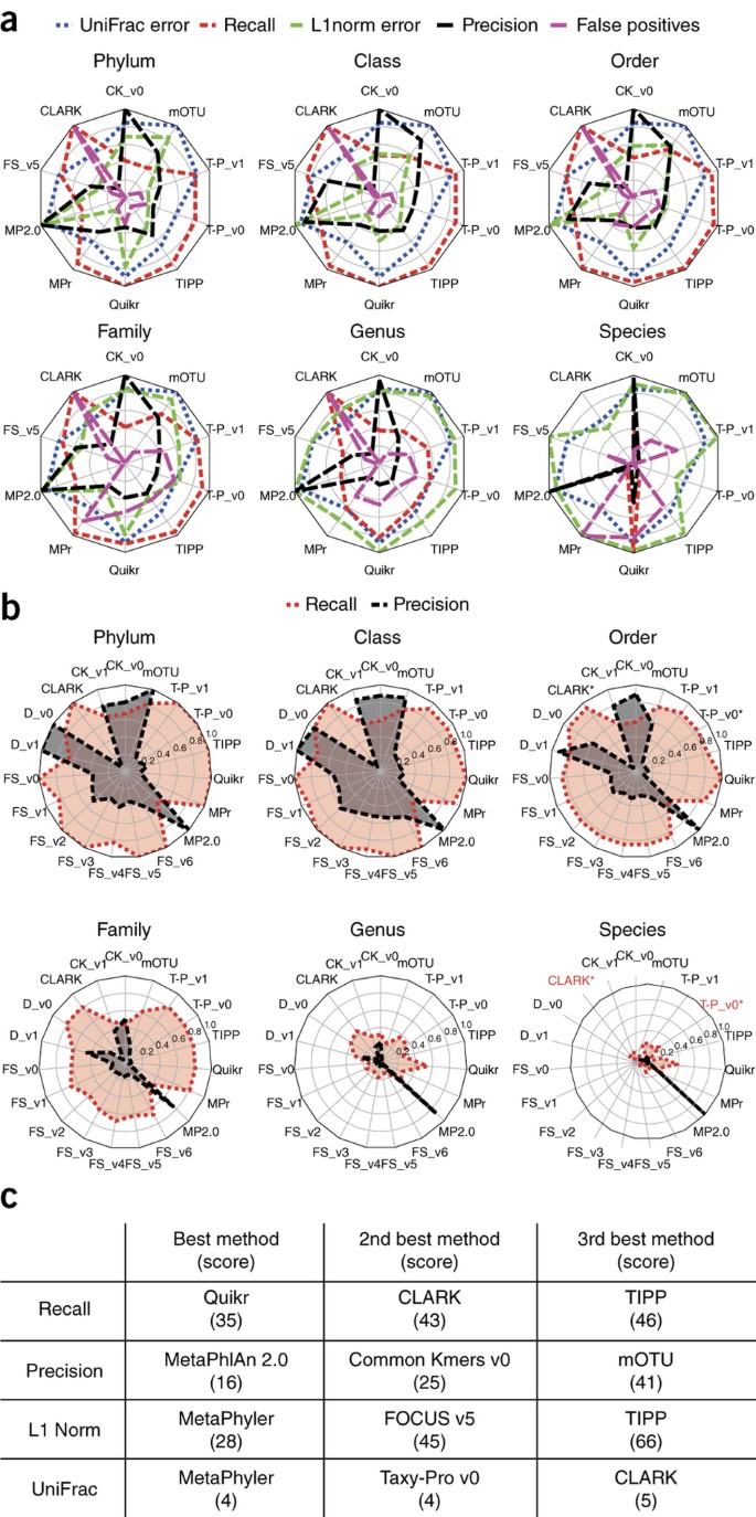
(a) Relative performance of profilers for different ranks and with different error metrics (weighted UniFrac, L1 norm, recall, precision and false positives) for the bacterial and archaeal portion of the first high-complexity sample. Each error metric was divided by its maximal value to facilitate viewing on the same scale and relative performance comparisons. (b) Absolute recall and precision for each profiler on the microbial (filtered) portion of the low-complexity data set across six taxonomic ranks. Red text and asterisk indicate methods for which no predictions at the corresponding taxonomic rank were returned. FS, FOCUS; T-P, Taxy-Pro; MP2.0, MetaPhlAn 2.0; MPr, MetaPhyler; CK, Common Kmers; D, DUDes. (c) Best scoring profilers using different performance metrics summed over all samples and taxonomic ranks to the genus level. A lower score indicates that a method was more frequently ranked highly for a particular metric. The maximum (worst) score for the UniFrac metric is 38 (18 + 11 + 9 profiling submissions for the low, medium and high-complexity data sets, respectively), while the maximum score for all other metrics is 190 (5 taxonomic ranks × (18 + 11 + 9) profiling submissions for the low, medium and high-complexity data sets, respectively).

Source data

Full size image

Quikr, CLARK, TIPP and Taxy-Pro had the highest recall, indicating their suitability for pathogen detection, where failure to identify an organism can have severe negative consequences. These were also among the least precise (Supplementary Figs. 29–33), typically owing to prediction of a large number of low-abundance organisms. MetaPhlAn 2.0 and Common Kmers were most precise, suggesting their use when many false positives would increase cost and effort in downstream analysis. MetaPhyler, FOCUS, TIPP, Taxy-Pro and CLARK best reconstructed relative abundances. On the basis of the average of precision and recall, over all samples and taxonomic ranks, Taxy-Pro version 0 (mean = 0.616), MetaPhlAn 2.0 (mean = 0.603) and DUDes version 0 (mean = 0.596) performed best.

Performance at different taxonomic ranks

Most profilers performed well only until the family level (Fig. 3a,b and Supplementary Figs. 29–33). Over all samples and programs at the phylum level, recall was 0.85 ± 0.19 (mean ± s.d.), and L1 norm, assessing abundance estimate quality at a particular rank, was 0.38 ± 0.28, both close to these metrics' optimal values (ranging from 1 to 0 and from 0 to 2, respectively), whereas precision was highly variable, at 0.53 ± 0.55. Precision and recall were high for several methods (DUDes, Common Kmers, mOTU and MetaPhlAn 2.0) until order rank. However, accurately reconstructing a taxonomic profile is still difficult below family level. Even for the low-complexity sample, only MetaPhlAn 2.0 maintained its precision at species level, while the largest recall at genus rank for the low-complexity sample was 0.55, for Quikr. Across all profilers and samples, there was a drastic decrease in average performance between the family and genus levels, of 0.48 ± 0.15% and 0.52 ± 0.18% for recall and precision, respectively, but comparatively little change between order and family levels, with a decrease of only 0.1 ± 0.07% and 0.1 ± 0.26%, for recall and precision, respectively. The other error metrics showed similar trends for all samples and methods (Fig. 3a and Supplementary Figs. 34–38).

Parameter settings and software versions

Several profilers were submitted with multiple parameter settings or versions (Supplementary Table 2). For some, this had little effect: for instance, the variance in recall among seven versions of FOCUS on the low-complexity sample at family level was only 0.002. For others, this caused large performance changes: for instance, one version of DUDes had twice the recall as that of another at phylum level on the pooled high-complexity sample (Supplementary Figs. 34–38). Notably, several developers submitted no results beyond a fixed taxonomic rank, as was the case for Taxy-Pro and Quikr. These submissions performed better than default program versions submitted by the CAMI team—indicating, not surprisingly, that experts can generate better results.

Performance for viruses and plasmids

We investigated the effect of including plasmids, viruses and other circular elements (Supplementary Table 6) in the gold-standard taxonomic profile (Supplementary Figs. 39–41). Here, the term 'filtered' indicates the gold standard without these data. The affected metrics were the abundance-based metrics (L1 norm at the superkingdom level and weighted UniFrac) and precision and recall (at the superkingdom level): all methods correctly detected Bacteria and Archaea, but only MetaPhlAn 2.0 and CLARK detected viruses in the unfiltered samples. Averaging over all methods and samples, L1 norm at the superkingdom level increased from 0.05, for the filtered samples, to 0.29, for the unfiltered samples. Similarly, the UniFrac metric increased from 7.21, for the filtered data sets, to 12.36, for the unfiltered data sets. Thus, the fidelity of abundance estimates decreased notably when viruses and plasmids were present.

Taxonomic profilers versus profiles from taxonomic binning

Using a simple coverage-approximation conversion algorithm, we derived profiles from the taxonomic binning results (Supplementary Note 1 and Supplementary Figs. 42–45). Overall, precision and recall of the taxonomic binners were comparable to that of the profilers. At the order level, the mean precision over all taxonomic binners was 0.60 (versus 0.40 for the profilers), and the mean recall was 0.82 (versus 0.86 for the profilers). MEGAN6 and PhyloPythiaS+ had better recall than the profilers at family level, though PhyloPythiaS+ precision was below that of Common Kmers and MetaPhlAn 2.0 as well as the binner taxator-tk (Supplementary Figs. 42 and 43), and—similarly to the profilers—recall also degraded below family level.

Abundance estimation at higher ranks was more problematic for the binners, as L1 norm error at the order level was 1.07 when averaged over all samples, whereas for the profilers it was only 0.68. Overall, though, the binners delivered slightly more accurate abundance estimates, as the binning average UniFrac metric was 7.03, whereas the profiling average was 7.23. These performance differences may be due in part to the gold-standard contigs used by the binners (except for MEGAN6), though Kraken is also often applied to raw reads, while the profilers used the raw reads.

Discussion

A lack of consensus about benchmarking data and evaluation metrics has complicated metagenomic software comparisons and their interpretation. To tackle this problem, the CAMI challenge engaged 19 teams with a series of benchmarks, providing performance data and guidance for applications, interpretation of results and directions for future work.

Assemblers using a range of _k_-mers clearly outperformed single _k_-mer assemblers (Supplementary Table 1). While the latter reconstructed only low-abundance genomes (with small _k_-mers) or high-abundance genomes (with large _k_-mers), using multiple _k_-mers substantially increased the recovered genome fraction. Two programs also reconstructed high-copy circular elements well, although none detected their circularities. An unsolved challenge for all programs is the assembly of closely related genomes. Notably, poor or failed assembly of these genomes will negatively affect subsequent contig binning and further complicate their study.

All genome binners performed well when no closely related strains were present. Taxonomic binners reconstructed taxon bins of acceptable quality down to the family rank (Supplementary Table 1). This leaves a gap in species and genus-level reconstruction—even when taxa are represented by single strains—that needs to be closed. Notably, taxonomic binners were more precise when reconstructing genomes than for species or genus bins, indicating that the decreased performance for low ranks is due partly to limitations of the reference taxonomy. A sequence-derived phylogeny might thus represent a more suitable reference framework for “phylogenetic” binning. When comparing the average taxon binner performance for taxa with similar surroundings in the SILVA and NCBI taxonomies to those with less agreement, we observed significant differences—primarily as a decrease in performance for low-ranking taxa in discrepant surroundings (Supplementary Note 1 and Supplementary Table 8). Thus, the use of SILVA might further improve taxon binning, but the lack of associated genome sequences represents a practical hurdle43. Another challenge for all programs is to deconvolute strain-level diversity. For the typical covariance of read coverage–based genome binners, it may require many more samples than those analyzed here (up to five) for satisfactory performance.

Despite variable performance, particularly for precision (Supplementary Table 1), most taxonomic profilers had good recall and low error in abundance estimates until family rank. The use of different classification algorithms, reference taxonomies, databases and information sources (for example, marker genes, _k_-mers) probably contributes to observed performance differences. To enable systematic analyses of their individual impacts, developers could provide configurable rather than hard-coded parameter options. Similarly to taxonomic binners, performance across all metrics dropped substantially below family level. When including plasmids and viruses, all programs gave worse abundance estimates, indicating a need for better analysis of data sets with such content, as plasmids are likely to be present, and viral particles are not always removed by size filtration44.

Additional programs can still be submitted and evaluated with the CAMI benchmarking platform. Currently, we are further automating the benchmarking and comparative result visualizations. As sequencing technologies such as long-read sequencing and metagenomics programs continue to evolve rapidly, CAMI will provide further challenges. We invite members of the community to contribute actively to future benchmarking efforts by CAMI.

Methods

Community involvement.

We organized public workshops, roundtables, hackathons and a research program around CAMI at the Isaac Newton Institute for Mathematical Sciences (Supplementary Fig. 46) to decide on the principles realized in data set generation and challenge design. To determine the most relevant metrics for performance evaluation, a meeting with developers of evaluation software and commonly used binning, profiling and assembly software was organized. Subsequently we created biobox containers implementing a range of commonly used performance metrics, including the ones decided to be most relevant in this meeting (Supplementary Table 9). Computational support for challenge participants was provided by the Pittsburgh Supercomputing Center.

Standardization and reproducibility.

For performance assessment, we developed several standards: we defined output formats for profiling and binning tools, for which no widely accepted standard existed. Second, we defined standards for submitting the software itself, along with parameter settings and required databases and implemented them in Docker container templates (bioboxes)10. These enable the standardized and reproducible execution of submitted programs from a particular category. Participants were encouraged to submit results together with their software in a Docker container following the bioboxes standard. In addition to 23 bioboxes submitted by challenge participants, we generated 13 other bioboxes and ran them on the challenge data sets (Supplementary Table 2), working with the developers to define the most suitable execution settings, if possible. For several submitted programs, bioboxes using default settings were created to compare performance with default and expert chosen parameter settings. If required, the bioboxes can be rerun on the challenge data sets.

Genome sequencing and assembly.

Draft genomes of 310 type strain isolates were generated for the Genomic Encyclopedia of Type Strains at the DOE Joint Genome Institute (JGI) using Illumina standard shotgun libraries and the Illumina HiSeq 2000 platform. All general aspects of library construction and sequencing performed at the JGI can be found at http://www.jgi.doe.gov. Raw sequence data were passed through DUK, a filtering program developed at JGI, which removes known Illumina sequencing and library preparation artifacts (L. Mingkun, A. Copeland and J. Han (Department of Energy Joint Genome Institute, personal communication). The genome sequences of isolates from culture collections are available in the JGI genome portal (Supplementary Table 10). Additionally, 488 isolates from the root and rhizosphere of Arabidopsis thaliana were sequenced8. All sequenced environmental genomes were assembled using the A5 assembly pipeline (default parameters, version 20141120)45 and are available for download at https://data.cami-challenge.org/participate. A quality control of all assembled genomes was performed on the basis of tetranucleotide content analysis and taxonomic analyses (Supplementary Note 1), resulting in 689 genomes that were used for the challenge (Supplementary Table 10). Furthermore, we generated 1.7 Mbp or 598 novel circular sequences of plasmids, viruses and other circular elements from multiple microbial community samples of rat cecum (Supplementary Note 1 and Supplementary Table 11).

Challenge data sets.

We simulated three metagenome data sets of different organismal complexities and sizes by generating 150-bp paired-end reads with an Illumina HighSeq error profile from the genome sequences of 689 newly sequenced bacterial and archaeal isolates and 598 sequences of plasmids, viruses and other circular elements (Supplementary Note 1, Supplementary Tables 3, 6 and 12 and Supplementary Figs. 47 and 48). These data sets represent common experimental setups and specifics of microbial communities. They consist of a 15-Gbp single sample data set from a low-complexity community with log normal abundance distribution (40 genomes and 20 circular elements), a 40-Gbp differential log normal abundance data set with two samples of a medium-complexity community (132 genomes and 100 circular elements) and long and short insert sizes, as well as a 75-Gbp time series data set with five samples from a high-complexity community with correlated log normal abundance distributions (596 genomes and 478 circular elements). The benchmark data sets had some notable properties; all included (i) species with strain-level diversity (Supplementary Fig. 47) to explore its effect on program performance; (ii) viruses, plasmids and other circular elements, for assessment of their impact on program performances; and (iii) genomes at different evolutionary distances to those in reference databases, to explore the effect of increasing taxonomic distance on taxonomic binning. Gold-standard assemblies, genome bin and taxon bin assignments and taxonomic profiles were generated for every individual metagenome sample and for the pooled samples of each data set.

Challenge organization.

The first CAMI challenge benchmarked software for sequence assembly, taxonomic profiling and (taxonomic) binning. To allow developers to familiarize themselves with the data types, biobox containers and in- and output formats, we provided simulated data sets from public data together with a 'standard of truth' before the start of the challenge. Reference data sets of RefSeq, NCBI bacterial genomes, SILVA46 and the NCBI taxonomy from 30 April 2014 were prepared for taxonomic binning and profiling tools, to enable performance comparisons for reference-based tools based on the same reference data sets. For future benchmarking of reference-based programs with the challenge data sets, it will be important to use these reference data sets, as the challenge data have subsequently become part of public reference data collections.

The CAMI challenge started on 27 March 2015 (Supplementary Figs. 46 and 49). Challenge participants had to register on the website to download the challenge data sets, and 40 teams registered at that time. They could then submit their predictions for all data sets or individual samples thereof. They had the option of providing an executable biobox implementing their software together with specifications of parameter settings and reference databases used. Submissions of assembly results were accepted until 20 May 2015. Subsequently, a gold-standard assembly was provided for all data sets and samples, which was suggested as input for taxonomic binning and profiling. This includes all genomic regions from the genome reference sequences and circular elements covered by at least one read in the pooled metagenome data sets or individual samples (Supplementary Note 1). Provision of this assembly gold standard allowed us to decouple the performance analyses of binning and profiling tools from assembly performance. Developers could submit their binning and profiling results until 18 July 2015.

Overall, 215 submissions representing 25 different programs were obtained for the three challenge data sets and samples, from initially 19 external teams and CAMI developers, 16 of which consented to publication (Supplementary Table 2). The genome data used to generate the simulated data sets was kept confidential until the end of the challenge and then released8. To ensure a more unbiased assessment, we required that challenge participants had no knowledge of the nature of the challenge data sets. Program results displayed in the CAMI portal were given anonymous names in an automated manner (only known to the respective challenge submitter) until a first consensus on performances was reached in the public evaluation workshop. In particular, this was considered relevant for evaluation of taxator-tk and PhyloPythiaS+, which were from the lab of one of the organizers (A.C.M.) but submitted without her involvement.

Evaluation metrics.

We briefly outline the metrics used to evaluate the four software categories. All metrics discussed, and several others, are described more in depth in Supplementary Note 1.

Assemblies. The assemblies were evaluated with MetaQUAST47 using a mapping of assemblies to the genome and circular element sequences of the benchmark data sets (Supplementary Table 4). As metrics, we focused on genome fraction and assembly size, the number of unaligned bases and misassemblies. Genome fraction measures the assembled percentage of an individual genome, assembly size denotes the total assembly length in bp (including misassemblies), and the number of misassemblies and unaligned bases are error metrics reflective of the assembly quality. Combined, they provide an indication of the program performance. For instance, although assembly size might be large, a high-quality assembly also requires the number of misassemblies and unaligned bases to be low. To assess how much metagenome data was included in each assembly, we also mapped all reads back to them.

Genome binning. We calculated completeness and purity for every bin relative to the genome with the highest number of base pairs in that bin. We measured the assignment accuracy for the portion of the assigned data by the programs with the ARI. This complements consideration of completeness and purity averaged over genome bins irrespectively of their sizes (Fig. 2c,d), as large bins contribute more than smaller bins in the evaluation. As not all programs assigned all data to genome bins, the ARI should be interpreted under consideration of the fraction of data assigned (Fig. 2a).

Taxonomic binning. As performance metrics, the average purity (precision) and completeness (recall) per taxon bin were calculated for individual ranks under consideration of the taxon assignment. In addition, we determined the overall classification accuracy for each data set, as measured by total assigned sequence length, and misclassification rate for all assignments. While the former two measures allow assessing performance averaged over bins, where all bins are treated equally, irrespective of their size, the latter are influenced by the taxonomic constitution, with large bins having a proportionally larger influence.

Taxonomic profiling. We determined abundance metrics (L1 norm and weighted UniFrac)48 and binary classification measures (recall and precision). The first two assess how well a particular method reconstructs the relative abundances in comparison to the gold standard, with the L1 norm using the sum of differences in abundances (ranges between 0 and 2) and UniFrac using differences weighted by distance in the taxonomic tree (ranges between 0 and 16). The binary classification metrics assess how well a particular method detects the presence or absence of an organism in comparison to the gold standard, irrespectively of their abundances. All metrics except the UniFrac metric (which is rank independent) are defined at each taxonomic rank. We also calculated the following summary statistic: for each metric, on each sample, we ranked the profilers by their performance. Each was assigned a score for its ranking (0 for first place among all tools at a particular taxonomic rank for a particular sample, 1 for second place, etc.). These scores were then added over the taxonomic ranks to the genus level and summed over the samples, to give a global performance score.

Data availability.

A Life Sciences Reporting Summary for this paper is available. The plasmid assemblies, raw data and metadata have been deposited in the European Nucleotide Archive (ENA) under accession number PRJEB20380. The challenge and toy data sets including the gold standard, the assembled genomes used to generate the benchmark data sets (Supplementary Table 10), NCBI and ARB public reference sequence collections without the benchmark data and the NCBI taxonomy version used for taxonomic binning and profiling are available in GigaDB under data set identifier (100344) and on the CAMI analysis site for download and within the benchmarking platform (https://data.cami-challenge.org/participate). Further information on the CAMI challenge, results and scripts is provided at https://github.com/CAMI-challenge/. Supplementary Tables 2 and 9 specify the Docker Hub locations of bioboxes for the evaluated programs and used metrics. Source data for Figures 1,2,3 are available online.

Additional information

Publisher's note: Springer Nature remains neutral with regard to jurisdictional claims in published maps and institutional affiliations.

Accession codes

Primary accessions

European Nucleotide Archive

References

1. Turaev, D. & Rattei, T. High definition for systems biology of microbial communities: metagenomics gets genome-centric and strain-resolved. Curr. Opin. Biotechnol. 39, 174–181 (2016).
   Article CAS PubMed Google Scholar
2. Mavromatis, K. et al. Use of simulated data sets to evaluate the fidelity of metagenomic processing methods. Nat. Methods 4, 495–500 (2007).
   Article CAS PubMed Google Scholar
3. Lindgreen, S., Adair, K.L. & Gardner, P.P. An evaluation of the accuracy and speed of metagenome analysis tools. Sci. Rep. 6, 19233 (2016).
   Article CAS PubMed PubMed Central Google Scholar
4. Marx, V. Microbiology: the road to strain-level identification. Nat. Methods 13, 401–404 (2016).
   Article CAS PubMed Google Scholar
5. Sangwan, N., Xia, F. & Gilbert, J.A. Recovering complete and draft population genomes from metagenome datasets. Microbiome 4, 8 (2016).
   Article PubMed PubMed Central Google Scholar
6. Yassour, M. et al. Natural history of the infant gut microbiome and impact of antibiotic treatment on bacterial strain diversity and stability. Sci. Transl. Med. 8, 343ra81 (2016).
   Article PubMed PubMed Central Google Scholar
7. Bendall, M.L. et al. Genome-wide selective sweeps and gene-specific sweeps in natural bacterial populations. ISME J. 10, 1589–1601 (2016).
   Article PubMed PubMed Central Google Scholar
8. Bai, Y. et al. Functional overlap of the Arabidopsis leaf and root microbiota. Nature 528, 364–369 (2015).
   Article CAS PubMed Google Scholar
9. Kashtan, N. et al. Single-cell genomics reveals hundreds of coexisting subpopulations in wild Prochlorococcus. Science 344, 416–420 (2014).
   Article CAS PubMed Google Scholar
10. Belmann, P. et al. Bioboxes: standardised containers for interchangeable bioinformatics software. Gigascience 4, 47 (2015).
    Article PubMed PubMed Central Google Scholar
11. Li, D., Liu, C.M., Luo, R., Sadakane, K. & Lam, T.W. MEGAHIT: an ultra-fast single-node solution for large and complex metagenomics assembly via succinct de Bruijn graph. Bioinformatics 31, 1674–1676 (2015).
    Article CAS PubMed Google Scholar
12. Chikhi, R. & Rizk, G. Space-efficient and exact de Bruijn graph representation based on a Bloom filter. Algorithms Mol. Biol. 8, 22 (2013).
    Article PubMed PubMed Central Google Scholar
13. Chapman, J.A. et al. Meraculous: de novo genome assembly with short paired-end reads. PLoS One 6, e23501 (2011).
    Article CAS PubMed PubMed Central Google Scholar
14. Gao, S., Sung, W.K. & Nagarajan, N. Opera: reconstructing optimal genomic scaffolds with high-throughput paired-end sequences. J. Comput. Biol. 18, 1681–1691 (2011).
    Article CAS PubMed PubMed Central Google Scholar
15. Boisvert, S., Laviolette, F. & Corbeil, J. Ray: simultaneous assembly of reads from a mix of high-throughput sequencing technologies. J. Comput. Biol. 17, 1519–1533 (2010).
    Article CAS PubMed PubMed Central Google Scholar
16. Cook, J.J. Scaling Short Read de novo DNA Sequence Assembly to Gigabase Genomes. PhD thesis, Univ. Illinois at Urbana–Champaign, (2011).
17. Konstantinidis, K.T. & Tiedje, J.M. Genomic insights that advance the species definition for prokaryotes. Proc. Natl. Acad. Sci. USA 102, 2567–2572 (2005).
    Article CAS PubMed PubMed Central Google Scholar
18. Lin, H.H. & Liao, Y.C. Accurate binning of metagenomic contigs via automated clustering sequences using information of genomic signatures and marker genes. Sci. Rep. 6, 24175 (2016).
    Article CAS PubMed PubMed Central Google Scholar
19. Wu, Y.W., Simmons, B.A. & Singer, S.W. MaxBin 2.0: an automated binning algorithm to recover genomes from multiple metagenomic datasets. Bioinformatics 32, 605–607 (2016).
    Article CAS PubMed Google Scholar
20. Kang, D.D., Froula, J., Egan, R. & Wang, Z. MetaBAT, an efficient tool for accurately reconstructing single genomes from complex microbial communities. PeerJ 3, e1165 (2015).
    Article PubMed PubMed Central Google Scholar
21. Strous, M., Kraft, B., Bisdorf, R. & Tegetmeyer, H.E. The binning of metagenomic contigs for microbial physiology of mixed cultures. Front. Microbiol. 3, 410 (2012).
    Article PubMed PubMed Central Google Scholar
22. Alneberg, J. et al. Binning metagenomic contigs by coverage and composition. Nat. Methods 11, 1144–1146 (2014).
    Article CAS PubMed Google Scholar
23. Gregor, I., Dröge, J., Schirmer, M., Quince, C. & McHardy, A.C. PhyloPythiaS+: a self-training method for the rapid reconstruction of low-ranking taxonomic bins from metagenomes. PeerJ 4, e1603 (2016).
    Article PubMed PubMed Central Google Scholar
24. Dröge, J., Gregor, I. & McHardy, A.C. Taxator-tk: precise taxonomic assignment of metagenomes by fast approximation of evolutionary neighborhoods. Bioinformatics 31, 817–824 (2015).
    Article PubMed Google Scholar
25. Huson, D.H. et al. MEGAN community edition—interactive exploration and analysis of large-scale microbiome sequencing data. PLoS Comput. Biol. 12, e1004957 (2016).
    Article PubMed PubMed Central Google Scholar
26. Wood, D.E. & Salzberg, S.L. Kraken: ultrafast metagenomic sequence classification using exact alignments. Genome Biol. 15, R46 (2014).
    Article PubMed PubMed Central Google Scholar
27. Miller, R.R., Montoya, V., Gardy, J.L., Patrick, D.M. & Tang, P. Metagenomics for pathogen detection in public health. Genome Med. 5, 81 (2013).
    Article PubMed PubMed Central Google Scholar
28. Arumugam, M. et al. Enterotypes of the human gut microbiome. Nature 473, 174–180 (2011).
    Article CAS PubMed PubMed Central Google Scholar
29. Human Microbiome Project Consortium. Structure, function and diversity of the healthy human microbiome. Nature 486, 207–214 (2012).
30. Koren, O. et al. A guide to enterotypes across the human body: meta-analysis of microbial community structures in human microbiome datasets. PLOS Comput. Biol. 9, e1002863 (2013).
    Article CAS PubMed PubMed Central Google Scholar
31. Ounit, R., Wanamaker, S., Close, T.J. & Lonardi, S. CLARK: fast and accurate classification of metagenomic and genomic sequences using discriminative k-mers. BMC Genomics 16, 236 (2015).
    Article PubMed PubMed Central Google Scholar
32. Koslicki, D. & Falush, D. MetaPalette: a k-mer Painting Approach for Metagenomic Taxonomic Profiling and Quantification of Novel Strain Variation. mSystems 1, e00020–16 (2016).
    Article PubMed PubMed Central Google Scholar
33. Piro, V.C., Lindner, M.S. & Renard, B.Y. DUDes: a top-down taxonomic profiler for metagenomics. Bioinformatics 32, 2272–2280 (2016).
    Article CAS PubMed Google Scholar
34. Silva, G.G., Cuevas, D.A., Dutilh, B.E. & Edwards, R.A. FOCUS: an alignment-free model to identify organisms in metagenomes using non-negative least squares. PeerJ 2, e425 (2014).
    Article PubMed PubMed Central Google Scholar
35. Segata, N. et al. Metagenomic microbial community profiling using unique clade-specific marker genes. Nat. Methods 9, 811–814 (2012).
    Article CAS PubMed PubMed Central Google Scholar
36. Liu, B., Gibbons, T., Ghodsi, M., Treangen, T. & Pop, M. Accurate and fast estimation of taxonomic profiles from metagenomic shotgun sequences. BMC Genomics 12 (Suppl. 2), S4 (2011).
    Article CAS PubMed PubMed Central Google Scholar
37. Sunagawa, S. et al. Metagenomic species profiling using universal phylogenetic marker genes. Nat. Methods 10, 1196–1199 (2013).
    Article CAS PubMed Google Scholar
38. Koslicki, D., Foucart, S. & Rosen, G. Quikr: a method for rapid reconstruction of bacterial communities via compressive sensing. Bioinformatics 29, 2096–2102 (2013).
    Article CAS PubMed Google Scholar
39. Koslicki, D. et al. ARK: Aggregation of Reads by _k_-Means for estimation of bacterial community composition. PLoS One 10, e0140644 (2015).
    Article PubMed PubMed Central Google Scholar
40. Chatterjee, S. et al. SEK: sparsity exploiting _k_-mer-based estimation of bacterial community composition. Bioinformatics 30, 2423–2431 (2014).
    Article CAS PubMed Google Scholar
41. Klingenberg, H., Aßhauer, K.P., Lingner, T. & Meinicke, P. Protein signature-based estimation of metagenomic abundances including all domains of life and viruses. Bioinformatics 29, 973–980 (2013).
    Article CAS PubMed PubMed Central Google Scholar
42. Nguyen, N.P., Mirarab, S., Liu, B., Pop, M. & Warnow, T. TIPP: taxonomic identification and phylogenetic profiling. Bioinformatics 30, 3548–3555 (2014).
    Article CAS PubMed PubMed Central Google Scholar
43. Balvočiūtė, M. & Huson, D.H. SILVA, RDP, Greengenes, NCBI and OTT—how do these taxonomies compare? BMC Genomics 18 (Suppl 2), 114 (2017).
    Article PubMed PubMed Central Google Scholar
44. Thomas, T., Gilbert, J. & Meyer, F. Metagenomics—a guide from sampling to data analysis. Microb. Inform. Exp. 2, 3 (2012).
    Article PubMed PubMed Central Google Scholar
45. Coil, D., Jospin, G. & Darling, A.E. A5-miseq: an updated pipeline to assemble microbial genomes from Illumina MiSeq data. Bioinformatics 31, 587–589 (2015).
    Article CAS PubMed Google Scholar
46. Pruesse, E. et al. SILVA: a comprehensive online resource for quality checked and aligned ribosomal RNA sequence data compatible with ARB. Nucleic Acids Res. 35, 7188–7196 (2007).
    Article CAS PubMed PubMed Central Google Scholar
47. Mikheenko, A., Saveliev, V. & Gurevich, A. MetaQUAST: evaluation of metagenome assemblies. Bioinformatics 32, 1088–1090 (2016).
    Article CAS PubMed Google Scholar
48. Lozupone, C. & Knight, R. UniFrac: a new phylogenetic method for comparing microbial communities. Appl. Environ. Microbiol. 71, 8228–8235 (2005).
    Article CAS PubMed PubMed Central Google Scholar

Download references

Acknowledgements

We thank C. Della Beffa, J. Alneberg, D. Huson and P. Grupp for their input, and the Isaac Newton Institute for Mathematical Sciences for its hospitality during the MTG program (supported by UK Engineering and Physical Sciences Research Council (EPSRC) grant EP/K032208/1). Sequencing at the US Department of Energy Joint Genome Institute was supported under contract DE-AC02-05CH11231. R.G.O. was supported by the Cluster of Excellence on Plant Sciences program of the Deutsche Forschungsgemeinschaft; A.E.D. and M.Z.D., through the Australian Research Council's Linkage Projects (LP150100912); J.A.V., by the European Research Council advanced grant (PhyMo); D.B., B.K.H.C. and N.N., by the Agency for Science, Technology and Research (A*STAR), Singapore; T.S.J., by the Lundbeck Foundation (project DK nr R44-A4384); L.H.H. by a VILLUM FONDEN Block Stipend on Mobilomics; and P.D.B. by the National Science Foundation (NSF, grant DBI-1458689). This work used the Bridges and Blacklight systems, supported by NSF awards ACI-1445606 and ACI-1041726, respectively, at the Pittsburgh Supercomputing Center (PSC), under the Extreme Science and Engineering Discovery Environment (XSEDE), supported by NSF grant OCI-1053575.

Author information

Author notes

1. Stephan Majda
   Present address: Department of Biodiversity, University of Duisburg-Essen, Essen, Germany
2. Yang Bai
   Present address: State Key Laboratory of Plant Genomics, Institute of Genetics and Developmental Biology, Beijing, China
3. Yang Bai
   Present address: Centre of Excellence for Plant and Microbial Sciences (CEPAMS), Beijing, China
4. Alexander Sczyrba, Peter Hofmann and Peter Belmann: These authors contributed equally to this work.

Authors and Affiliations

1. Faculty of Technology, Bielefeld University, Bielefeld, Germany
   Alexander Sczyrba, Peter Belmann & Andreas Bremges
2. Center for Biotechnology, Bielefeld University, Bielefeld, Germany
   Alexander Sczyrba, Peter Belmann & Andreas Bremges
3. Formerly Department of Algorithmic Bioinformatics, Heinrich Heine University (HHU), Duesseldorf, Germany
   Peter Hofmann, Johannes Dröge, Ivan Gregor, Stephan Majda, Jessika Fiedler, Eik Dahms, Ruben Garrido-Oter & Alice C McHardy
4. Department of Computational Biology of Infection Research, Helmholtz Centre for Infection Research (HZI), Braunschweig, Germany
   Peter Hofmann, Peter Belmann, Stefan Janssen, Johannes Dröge, Ivan Gregor, Jessika Fiedler, Eik Dahms, Andreas Bremges, Adrian Fritz, Ruben Garrido-Oter, Fernando Meyer & Alice C McHardy
5. Braunschweig Integrated Centre of Systems Biology (BRICS), Braunschweig, Germany
   Peter Hofmann, Peter Belmann, Johannes Dröge, Ivan Gregor, Eik Dahms, Andreas Bremges, Adrian Fritz, Ruben Garrido-Oter, Fernando Meyer & Alice C McHardy
6. Mathematics Department, Oregon State University, Corvallis, Oregon, USA
   David Koslicki
7. Department of Pediatrics, University of California, San Diego, California, USA
   Stefan Janssen
8. Department of Computer Science and Engineering, University of California, San Diego, California, USA
   Stefan Janssen
9. German Center for Infection Research (DZIF), partner site Hannover-Braunschweig, Braunschweig, Germany
   Andreas Bremges
10. Department of Plant Microbe Interactions, Max Planck Institute for Plant Breeding Research, Cologne, Germany
    Ruben Garrido-Oter, Yang Bai & Paul Schulze-Lefert
11. Cluster of Excellence on Plant Sciences (CEPLAS),
    Ruben Garrido-Oter, Paul Schulze-Lefert & Alice C McHardy
12. Department of Environmental Science, Section of Environmental microbiology and Biotechnology, Aarhus University, Roskilde, Denmark
    Tue Sparholt Jørgensen & Lars Hestbjerg Hansen
13. Department of Microbiology, University of Copenhagen, Copenhagen, Denmark
    Tue Sparholt Jørgensen & Søren J Sørensen
14. Department of Science and Environment, Roskilde University, Roskilde, Denmark
    Tue Sparholt Jørgensen
15. Department of Energy, Joint Genome Institute, Walnut Creek, California, USA
    Nicole Shapiro, Jeff L Froula, Zhong Wang, Robert Egan, Dongwan Don Kang, Michael D Barton, Nikos C Kyrpides, Tanja Woyke & Edward M Rubin
16. Pittsburgh Supercomputing Center, Carnegie Mellon University, Pittsburgh, Pennsylvania, USA
    Philip D Blood
17. Center for Algorithmic Biotechnology, Institute of Translational Biomedicine, Saint Petersburg State University, Saint Petersburg, Russia
    Alexey Gurevich
18. Department of Microbiology and Ecosystem Science, University of Vienna, Vienna, Austria
    Dmitrij Turaev & Thomas Rattei
19. The ithree institute, University of Technology Sydney, Sydney, New South Wales, Australia
    Matthew Z DeMaere & Aaron E Darling
20. Department of Computer Science, Research Center in Computer Science (CRIStAL), Signal and Automatic Control of Lille, Lille, France
    Rayan Chikhi
21. National Centre of the Scientific Research (CNRS), Rennes, France
    Rayan Chikhi & Dominique Lavenier
22. Department of Computational and Systems Biology, Genome Institute of Singapore, Singapore
    Niranjan Nagarajan, Burton K H Chia & Bertrand Denis
23. Department of Microbiology and Infection, Warwick Medical School, University of Warwick, Coventry, UK
    Christopher Quince
24. Department of Computer Science, University of Tuebingen, Tuebingen, Germany
    Monika Balvočiūtė
25. Intel Corporation, Hillsboro, Oregon, USA
    Jeffrey J Cook
26. GenScale—Bioinformatics Research Team, Inria Rennes—Bretagne Atlantique Research Centre, Rennes, France
    Charles Deltel, Claire Lemaitre & Pierre Peterlongo
27. Institute of Research in Informatics and Random Systems (IRISA), Rennes, France
    Charles Deltel, Claire Lemaitre, Pierre Peterlongo, Guillaume Rizk & Dominique Lavenier
28. Department of Molecular Infection Biology, Helmholtz Centre for Infection Research, Braunschweig, Germany
    Michael Beckstette
29. Algorizk–IT consulting and software systems, Paris, France
    Guillaume Rizk
30. Joint BioEnergy Institute, Emeryville, California, USA
    Yu-Wei Wu & Steven W Singer
31. Graduate Institute of Biomedical Informatics, College of Medical Science and Technology, Taipei Medical University, Taipei, Taiwan
    Yu-Wei Wu
32. Biological Systems and Engineering Division, Lawrence Berkeley National Laboratory, Berkeley, California, USA
    Steven W Singer
33. School of Computational Science and Engineering, Georgia Institute of Technology, Atlanta, Georgia, USA
    Chirag Jain
34. Energy Engineering and Geomicrobiology, University of Calgary, Calgary, Alberta, Canada
    Marc Strous
35. Department of Bioinformatics, Institute for Microbiology and Genetics, University of Goettingen, Goettingen, Germany
    Heiner Klingenberg & Peter Meinicke
36. Genevention GmbH, Goettingen, Germany
    Thomas Lingner
37. Institute of Population Health Sciences, National Health Research Institutes, Zhunan Town, Taiwan
    Hsin-Hung Lin & Yu-Chieh Liao
38. Computational Science Research Center, San Diego State University, San Diego, California, USA
    Genivaldo Gueiros Z Silva, Daniel A Cuevas & Robert A Edwards
39. Boyce Thompson Institute for Plant Research, New York, New York, USA
    Surya Saha
40. Research Group Bioinformatics (NG4), Robert Koch Institute, Berlin, Germany
    Vitor C Piro & Bernhard Y Renard
41. Coordination for the Improvement of Higher Education Personnel (CAPES) Foundation, Ministry of Education of Brazil, Brasília, Brazil
    Vitor C Piro
42. Center for Bioinformatics and Computational Biology, University of Maryland, College Park, Maryland, USA
    Mihai Pop
43. Department of Computer Science, University of Maryland, College Park, Maryland, USA
    Mihai Pop
44. School of Biology, Newcastle University, Newcastle upon Tyne, UK
    Hans-Peter Klenk
45. Leibniz Institute DSMZ—German Collection of Microorganisms and Cell Cultures, Braunschweig, Germany
    Markus Göker
46. Institute of Microbiology, ETH Zurich, Zurich, Switzerland
    Julia A Vorholt

Authors

1. Alexander Sczyrba
   You can also search for this author inPubMed Google Scholar
2. Peter Hofmann
   You can also search for this author inPubMed Google Scholar
3. Peter Belmann
   You can also search for this author inPubMed Google Scholar
4. David Koslicki
   You can also search for this author inPubMed Google Scholar
5. Stefan Janssen
   You can also search for this author inPubMed Google Scholar
6. Johannes Dröge
   You can also search for this author inPubMed Google Scholar
7. Ivan Gregor
   You can also search for this author inPubMed Google Scholar
8. Stephan Majda
   You can also search for this author inPubMed Google Scholar
9. Jessika Fiedler
   You can also search for this author inPubMed Google Scholar
10. Eik Dahms
    You can also search for this author inPubMed Google Scholar
11. Andreas Bremges
    You can also search for this author inPubMed Google Scholar
12. Adrian Fritz
    You can also search for this author inPubMed Google Scholar
13. Ruben Garrido-Oter
    You can also search for this author inPubMed Google Scholar
14. Tue Sparholt Jørgensen
    You can also search for this author inPubMed Google Scholar
15. Nicole Shapiro
    You can also search for this author inPubMed Google Scholar
16. Philip D Blood
    You can also search for this author inPubMed Google Scholar
17. Alexey Gurevich
    You can also search for this author inPubMed Google Scholar
18. Yang Bai
    You can also search for this author inPubMed Google Scholar
19. Dmitrij Turaev
    You can also search for this author inPubMed Google Scholar
20. Matthew Z DeMaere
    You can also search for this author inPubMed Google Scholar
21. Rayan Chikhi
    You can also search for this author inPubMed Google Scholar
22. Niranjan Nagarajan
    You can also search for this author inPubMed Google Scholar
23. Christopher Quince
    You can also search for this author inPubMed Google Scholar
24. Fernando Meyer
    You can also search for this author inPubMed Google Scholar
25. Monika Balvočiūtė
    You can also search for this author inPubMed Google Scholar
26. Lars Hestbjerg Hansen
    You can also search for this author inPubMed Google Scholar
27. Søren J Sørensen
    You can also search for this author inPubMed Google Scholar
28. Burton K H Chia
    You can also search for this author inPubMed Google Scholar
29. Bertrand Denis
    You can also search for this author inPubMed Google Scholar
30. Jeff L Froula
    You can also search for this author inPubMed Google Scholar
31. Zhong Wang
    You can also search for this author inPubMed Google Scholar
32. Robert Egan
    You can also search for this author inPubMed Google Scholar
33. Dongwan Don Kang
    You can also search for this author inPubMed Google Scholar
34. Jeffrey J Cook
    You can also search for this author inPubMed Google Scholar
35. Charles Deltel
    You can also search for this author inPubMed Google Scholar
36. Michael Beckstette
    You can also search for this author inPubMed Google Scholar
37. Claire Lemaitre
    You can also search for this author inPubMed Google Scholar
38. Pierre Peterlongo
    You can also search for this author inPubMed Google Scholar
39. Guillaume Rizk
    You can also search for this author inPubMed Google Scholar
40. Dominique Lavenier
    You can also search for this author inPubMed Google Scholar
41. Yu-Wei Wu
    You can also search for this author inPubMed Google Scholar
42. Steven W Singer
    You can also search for this author inPubMed Google Scholar
43. Chirag Jain
    You can also search for this author inPubMed Google Scholar
44. Marc Strous
    You can also search for this author inPubMed Google Scholar
45. Heiner Klingenberg
    You can also search for this author inPubMed Google Scholar
46. Peter Meinicke
    You can also search for this author inPubMed Google Scholar
47. Michael D Barton
    You can also search for this author inPubMed Google Scholar
48. Thomas Lingner
    You can also search for this author inPubMed Google Scholar
49. Hsin-Hung Lin
    You can also search for this author inPubMed Google Scholar
50. Yu-Chieh Liao
    You can also search for this author inPubMed Google Scholar
51. Genivaldo Gueiros Z Silva
    You can also search for this author inPubMed Google Scholar
52. Daniel A Cuevas
    You can also search for this author inPubMed Google Scholar
53. Robert A Edwards
    You can also search for this author inPubMed Google Scholar
54. Surya Saha
    You can also search for this author inPubMed Google Scholar
55. Vitor C Piro
    You can also search for this author inPubMed Google Scholar
56. Bernhard Y Renard
    You can also search for this author inPubMed Google Scholar
57. Mihai Pop
    You can also search for this author inPubMed Google Scholar
58. Hans-Peter Klenk
    You can also search for this author inPubMed Google Scholar
59. Markus Göker
    You can also search for this author inPubMed Google Scholar
60. Nikos C Kyrpides
    You can also search for this author inPubMed Google Scholar
61. Tanja Woyke
    You can also search for this author inPubMed Google Scholar
62. Julia A Vorholt
    You can also search for this author inPubMed Google Scholar
63. Paul Schulze-Lefert
    You can also search for this author inPubMed Google Scholar
64. Edward M Rubin
    You can also search for this author inPubMed Google Scholar
65. Aaron E Darling
    You can also search for this author inPubMed Google Scholar
66. Thomas Rattei
    You can also search for this author inPubMed Google Scholar
67. Alice C McHardy
    You can also search for this author inPubMed Google Scholar

Contributions

R.C., N.N., C.Q., B.K.H.C., B.D., J.L.F., Z.W., R.E., D.D.K., J.J.C., C.D., C.L., P.P., G.R., D.L., Y.-W.W., S.W.S., C.J., M.S., H.K., P.M., T.L., H.-H.L., Y.-C.L., G.G.Z.S., D.A.C., R.A.E., S.S., V.C.P., B.Y.R., D.K., J.D. and I.G. participated in challenge; P.S.-L., J.A.V., Y.B., T.S.J., L.H.H., S.J.S., N.C.K., E.M.R., T.W., H.-P.K., M.G. and N.S. generated and contributed data; P.H., S.M., J.F., E.D., D.T., M.Z.D., A.S., A.B., A.E.D., T.R. and A.C.M. generated benchmark data sets; P.B. implemented the benchmarking platform; M. Beckstette and P.D.B. provided computational support; D.K., P.H., S.J., J.D., I.G., R.G.-O., C.Q., A.F., F.M., P.B., M.D.B., M. Balvočiūtė and A.G. implemented benchmarking metrics and bioboxes and performed evaluations; D.K., A.S., A.C.M., C.Q., J.D., P.H., T.S.J., D.D.K., Y.-W.W., A.B., A.F., R.C., M.P. and P.B. interpreted results with comments from many authors; A.C.M., A.S. and D.K. wrote the paper with comments from many authors; A.S., T.R. and A.C.M. conceived research with input from many authors.

Corresponding authors

Correspondence toAlexander Sczyrba or Alice C McHardy.

Ethics declarations

Competing interests

The authors declare no competing financial interests.

Supplementary information

Supplementary Text and Figures

Supplementary Figures 1–49 and Supplementary Note 1. (PDF 13234 kb)

Life Sciences Reporting Summary

Life Sciences Reporting Summary. (PDF 128 kb)

Supplementary Table 1

Computational metagenomics programs evaluated in the CAMI challenge. (XLSX 12 kb)

Supplementary Table 2

Overview over program submissions, their parameter settings and availability in bioboxes. (XLSX 41 kb)

Supplementary Table 3

Overview of the CAMI challenge data sets. (XLSX 11 kb)

Supplementary Table 4

Combined assembly metrics for each assembler or assembly pipeline as determined by MetaQUAST for the pooled high-complexity data sets (including contigs of at least 500 bp). (XLSX 12 kb)

Supplementary Table 5

Precision and recall for genome binners by genome, for all genomes. (XLSX 12 kb)

Supplementary Table 6

Taxonomic composition of the three challenge data sets. (XLSX 11 kb)

Supplementary Table 7

Full results of scoring methods using different performance metrics summed over all samples and taxonomic ranks. (XLSX 10 kb)

Supplementary Table 8

Spearman correlation coefficients, P values, and permutation test values computed from the sum of precision and recall averaged over all participating taxon binning tools and all data sets for individual taxa versus the dissimilarities of the taxon descending lineages and surroundings in the NCBI versus the SILVA taxonomy. (XLSX 10 kb)

Supplementary Table 9

Bioboxes implementing the CAMI benchmarking metrics used to evaluate the program results of the CAMI challenge. (XLSX 12 kb)

Supplementary Table 10

All the newly sequenced genomes used as reference genomes for the CAMI challenge. (XLSX 36 kb)

Supplementary Table 11

Pfam domains used for categorization of circular elements. (XLSX 15 kb)

Supplementary Table 12

Taxonomic composition of the challenge data sets in % bp. (XLSX 43 kb)

Source data

Rights and permissions

This work is licensed under a Creative Commons Attribution 4.0 International (CC BY 4.0) License. The images or other third party material in this article are included in the article’s Creative Commons license, unless indicated otherwise in the credit line; if the material is not included under the Creative Commons license, users will need to obtain permission from the license holder to reproduce the material. To view a copy of this license, visit http://creativecommons.org/licenses/by/4.0/

Reprints and permissions

About this article

Cite this article

Sczyrba, A., Hofmann, P., Belmann, P. et al. Critical Assessment of Metagenome Interpretation—a benchmark of metagenomics software.Nat Methods 14, 1063–1071 (2017). https://doi.org/10.1038/nmeth.4458

Download citation

• Received: 29 December 2016
• Accepted: 25 August 2017
• Published: 02 October 2017
• Issue Date: 01 November 2017
• DOI: https://doi.org/10.1038/nmeth.4458