Quantifying the Behavior of Stock Correlations Under Market Stress (original) (raw)
Abstract
Understanding correlations in complex systems is crucial in the face of turbulence, such as the ongoing financial crisis. However, in complex systems, such as financial systems, correlations are not constant but instead vary in time. Here we address the question of quantifying state-dependent correlations in stock markets. Reliable estimates of correlations are absolutely necessary to protect a portfolio. We analyze 72 years of daily closing prices of the 30 stocks forming the Dow Jones Industrial Average (DJIA). We find the striking result that the average correlation among these stocks scales linearly with market stress reflected by normalized DJIA index returns on various time scales. Consequently, the diversification effect which should protect a portfolio melts away in times of market losses, just when it would most urgently be needed. Our empirical analysis is consistent with the interesting possibility that one could anticipate diversification breakdowns, guiding the design of protected portfolios.
Introduction
Wild fluctuations in stock prices1,2,3,4,5,6,7,8 continue to have a huge impact on the world economy and the personal fortunes of millions, shedding light on the complex nature of financial and economic systems. For these systems, a truly gargantuan amount of pre-existing precise financial market data9,10,11 complemented by new big data ressources12,13,14,15 is available for analyses.
The complex mechanisms of financial market moves can lead to sudden trend switches16,17,18 in a number of stocks. Such sudden trend switches can occur in a synchronized fashion, in a large number of stocks simultaneously, or in an unsynchronized fashion, affecting only a few stocks at the same time.
Diversification in stock markets refers to the reduction of portfolio risk caused by the investment in a variety of stocks. If stock prices do not move up and down in perfect synchrony, a diversified portfolio will have less risk than the weighted average risk of its constituent stocks19,20. Hence it should be possible to reduce risk in price of individual stocks by the combination of an appropriate set of stocks. To identify such an appropriate set of stocks with anti-correlated price time series, the assumption mostly used is that the correlations among stocks are constant over time21,22,23,24,25,26. This widely used assumption is also the basis for the determination of capital requirements of financial institutions that usually own a huge variety of constituents belonging to different asset classes.
Recent studies building on the availability of huge and detailed data sets of financial markets have analyzed and modeled the static and dynamic behavior of this very complex system27,28,29,30,31,32,33,34,35,36,37,38,39, suggesting that financial markets are governed by systemic shifts and display non-equilibrium properties.
A very well known stylized fact of financial markets is the leverage effect, a term coined by Black to describe the negative correlation between past price returns and future realized volatilities in stock markets. According to Reigneron et al.40, the index leverage effect can be decomposed into a volatility effect and a correlation effect. In the course of recent financial market crises, this effect has regained center stage and the work of different groups has focused on uncovering its true nature40,41,42,43,44,45,46). Reigneron et al. analyzed daily returns of six indices from 2000 to 2010 and found that a downward index trends increase the average correlation between stocks, as quantified by measurements of eigenvalues of the conditional correlation matrix. They suggest that a quadratic term should be included to the linear regressions of the dependence of mean correlation on the index return the previous day.
Here, we will expand on these results utilizing 72 years of trading of the 30 Dow Jones industrial average (DJIA) components (see also47,48). Using this financial data set we will quantify state-dependent stock market correlations and analyze how they vary in face of dramatic market losses. In such “stress” scenarios, reliable correlations are most needed to protect the value of a portfolio against losses.
Results
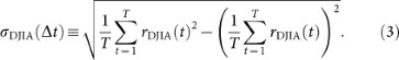
To quantify state-dependent correlations, we analyze historical daily closing prices of the N ≡ 30 components of the DJIA over 72 years, from 15 March 1939 until 31 December 2010, which can be downloaded as a Supplementary Dataset . During these T ≡ 18596 trading days, various adjustments of the DJIA occurred. We explicitly consider an adjustment of the index when one of the 30 stocks is removed from the index and replaced by a new stock in order to ensure that we accurately reproduce the index value of the DJIA at each trading day (Fig. 1).
Figure 1
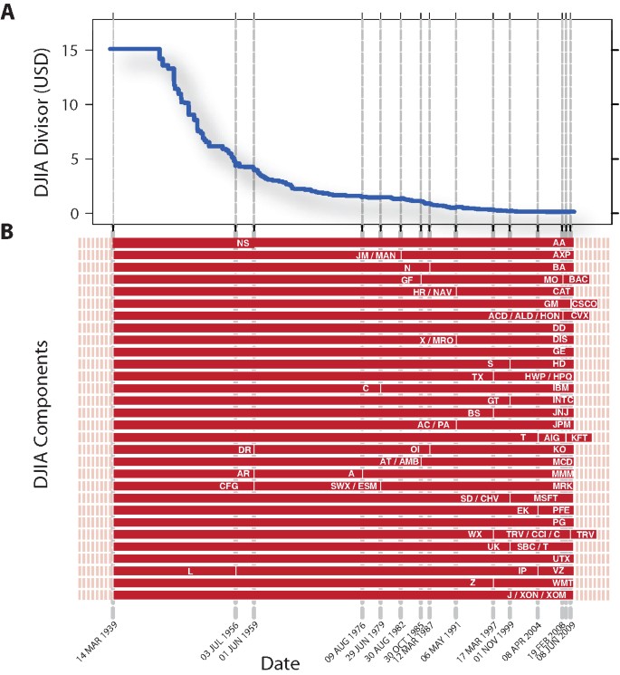
The alternative text for this image may have been generated using AI.
Index components of the Dow Jones Industrial Average (DJIA).
(A) To calculate the index value of the DJIA, we determine the sum of prices of all 30 stocks belonging to the index and divide them by the depicted “DJIA Divisor”. Adjustments of this divisor ensure that various corporate actions such as stock splits do not affect the index value. (B) We analyze DJIA values and prices of all index components for 72 years from March 15, 1939 until December 31, 2010. Vertical dashed lines correspond to events in which at least one stock was removed from the index and replaced by another stock. The index changes are explicitly taken into account to ensure that the dataset, comprising 18,596 trading days, accurately reflects all 30 daily closing prices needed for the index calculation. We use current and historical ticker symbols to abbreviate company names[50](/articles/srep00752#ref-CR50 "The URL http://en.wikipedia.org/wiki/Ticker_symbol
was retrieved on 23rd October 2011.").To calculate the official index value _p_DJIA, the sum of prices of all 30 stocks is divided by a normalization factor _d_DJIA, known as the DJIA divisor. The DJIA divisor anticipates index jumps caused by effects of stock splits, bonus issues, dividends payouts or replacements of individual index components keeping the index value consistent (Fig. 1A). Consequently, the index value of the DJIA at day t is given by
where p i(t) reflects the price of DJIA component i at day t in units of USD and where t is measured in units of trading days. The normalization factor _d_DJIA is also measured in units of USD. Consequently, the value of the DJIA is dimensionless. Due to changes in the components of the DJIA, a component i does not necessarily reflect prices of one stock only. A subscript i is also used for a component's predecessor or successor.
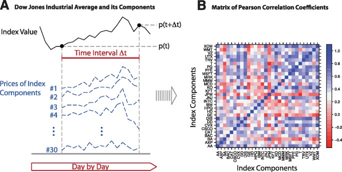
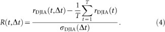
To quantify state-dependent correlations, we calculate the mean value of Pearson product-moment correlation coefficients49 among all DJIA components in a time interval comprising Δ_t_ trading days each (Fig. 2). In each time interval comprising Δ_t_ trading day, we determine correlation coefficients for all pairs of N ≡ 30 stocks. From these correlation coefficients, we calculate their mean value for each time interval separately.
Figure 2
The alternative text for this image may have been generated using AI.
Visualization of the analysis method.
(A) For a time interval of Δ_t_ trading days, we calculate for the index the price return log(p_DJIA(t + Δ_t))/log(_p_DJIA(t)) in this interval. (B) We determine the Pearson correlation coefficients of all pairs of all 30 DJIA components depicted in a matrix of correlation coefficients. Ticker symbols are used to abbreviate company names in this example. We calculate the mean correlation coefficient by averaging over all non-diagonal elements of this matrix.
We relate mean correlation coefficients to corresponding market states, which we quantify by DJIA index returns for time intervals starting at trading day t and ending at trading day t + Δ_t_,
We normalize the time series of DJIA index returns, r_DJIA(t, Δ_t), by its standard deviation, σDJIA(Δ_t_), defined as
The normalized time series of DJIA index returns, R(t, Δ_t_), is given by
In each time interval comprising Δ_t_ trading days, we calculate a local correlation matrix consisting of Pearson correlation coefficients49 capturing the dependencies among individual stock returns. Time-dependent returns of an individual stock i are given by
In a Δ_t_ trading day interval, we calculate a correlation coefficient between return time series of stock i and return time series of stock j by
with the standard deviation of return time series i determined in the same time interval comprising Δ_t_ trading days defined as
The mean correlation coefficient of all DJIA components is given by the mean of all non-diagonal matrix elements of c i,j
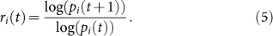
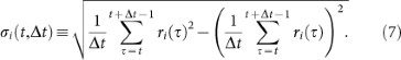
Figure 3A depicts the relationship between normalized DJIA index return and corresponding mean correlation coefficient capturing the dependency amoung its components. Figure 3B depicts both normalized DJIA index returns and mean correlation coefficients which are used in our analysis for Δ_t_ = 10 days. Negative index returns tend to come with stronger correlation coefficients than positive index returns (Fig. 3A). Results for different time intervals Δ_t_ collapse into one single curve, suggesting a universal relationship.
Figure 3
The alternative text for this image may have been generated using AI.
Quantification of state-dependent correlations among index components.
(A) Graphs reflect the relationship between the average correlation coefficient C among stocks belonging to the Dow Jones Industrial Average and its normalized return in intervals of Δ_t_ trading days. The mean correlation coefficient shows a striking, non-constant behavior, with a minimum between 0 and +1 standard deviations reflecting typical market conditions. For the range of all Δ_t_ values analyzed, we find the data collapse onto a single line. Corresponding error bars are shown in Fig. 4A. The data collapse suggests that the striking increase of the mean correlation coefficient for positive and negative values of the normalized index return is independent of the time interval Δ_t_. The largest mean correlation coefficients coincide with the most negative index returns. (B) Normalized DJIA returns, R(t, Δ_t_) and mean correlation coefficients, C(t, Δ_t_), shown for Δ_t_ = 10 days. For both time series, we reject the null hypothesis of non-stationarity on the basis of results from the Augmented Dickey-Fuller test. For R(t, Δ_t_ = 10), we obtain DF = −24.28, p < 0.01, while for C(t, Δ_t_ = 10) we obtain DF = −13.45, p < 0.01.
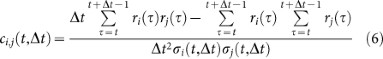
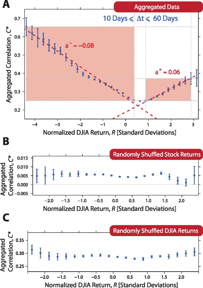
To quantify the relationship between normalized index return and average correlation, we aggregate mean correlation coefficients for different values of Δ_t_ ranging from 10 trading days to 60 trading days (Fig. 4),
We find consistency with two linear relationships quantifying the increase of the aggregated correlation C+ for positive index return R and the aggregated correlation _C_− for negative index return R,

with a+ = 0.064 ± 0.002 and b+ = 0.188 ± 0.004 (_p_-value < 0.001) quantifies the right part in Fig. 4A. The aggregatated correlations,

with _a_− = −0.085 ± 0.002 and _b_− = 0.267 ± 0.005 (_p_–value < 0.001) quantifies the left part in Fig. 4A. The larger is a negative or positive DJIA return the larger is the corresponding mean correlation. In contrast, a reference scenario of randomly shuffled stock returns leads to a constant relationship (Fig. 4B), supporting our findings in Fig. 4A. However, this method destroys all correlations of this complex financial system and not only the link between aggregated correlation C* and normalized index returns R. As an additional test, we use non-shuffled time series of underlying stock returns for our analysis and randomly shuffle the DJIA return time series only (Fig. 4C). We find that the linear relationships reported in Fig. 4A also vanishes in this scenario highlighting the robustness of our findings.
Figure 4
The alternative text for this image may have been generated using AI.
Quantification of the aggregated correlation.
(A) Utilizing the data collapse reported in Fig. 3, we aggregate in each bin of the graph the mean correlation coefficients for 10 days ≤ Δ_t_ ≤ 60 days. Error bars are plotted depicting −1 and +1 standard deviations around the mean of the mean correlation values included in each bin. The increase of the aggregated correlation C* for positive and negative index returns is consistent with two linear relationships: C* = a+R + b+ with a+ = 0.064 ± 0.002 and b+ = 0.188 ± 0.004 (p – value < 0.001) quantifies the right part. C* = a_−_R + _b_− with _a_− = −0.085 ± 0.002 and b_− = 0.267 ± 0.005 (p – value < 0.001). The red colored regions are used to obtain the coefficients. In order to reduce noise, the range of normalized DJIA returns is restricted to bin values occurring, on average, more than 10 times for individual Δ_t intervals. (B) By randomly shuffling time series of daily returns for each stock individually, we test the robustness of the relationship and find that the linear relationships reported in (A) disappear, supporting our findings. (C) We use non-shuffled time series of underlying stock returns for an additional parallel analysis with randomly shuffled DJIA returns. The above linear relationships also vanish in this test scenario underlining the robustness of our findings.
Our findings are qualitatively consistent with results reported in previous work40,43,44 but quantitatively different. Instead of linear relationships, Reigneron et al.40 suggest that a quadratic term should be included in the linear regressions of the dependence of mean correlation on the index return on the previous day.
Discussion
In summary, we find a universal relationship between the mean correlation among DJIA components which can be considered as a stock market portfolio and the normalized returns of this portfolio. This suggests that a “diversification breakdown” tends to occur when stable correlations are most needed for portfolio protection. Our findings, which are qualitatively consistent with earlier findings42,44 but quantitatively different, could be used to anticipate changes in mean correlation of portfolios when financial markets are suffering significant losses. This would enable a more accurate assessment of the risk of losses. Thus, we suggest that in order to anticipate underlying correlation risks the possibility exists to hedge index derivatives. Our results could also shed light on why correlation risks in mortgage bundles were underestimated at the beginning of the recent financial crisis. Future work will build upon the relationship quantified here to uncover the underlying mechanisms governing this phenomenon.
References
- O'Hara, M. Market Microstructure Theory (Blackwell, Cambridge, Massachusetts, 1995).
- Bouchaud, J. P. & Potters, M. Theory of Financial Risk and Derivative Pricing: From Statistical Physics to Risk Management (Cambridge University press, 2003).
- Sornette, D. Why stock markets crash: critical events in complex financial systems (Princeton University Press, 2004).
- Volt, J. The statistical mechanics of financial markets (Springer Verlag, 2005).
- Sinha, S., Chatterjee, A., Chakraborti, A. & Chakrabarti, B. K. Econophysics: an introduction (Wiley-VCH, 2010).
- Preis, T. Ökonophysik: Die Physik des Finanzmarktes (Gabler Verlag, 2011).
- Abergel, F., Chakrabarti, B. K., Chakrabarti, A. & Mitra, M. Econophysics of Order-driven Markets (Springer Verlag, 2011).
- Takayasu, H. ed., Practical Fruits of Econophysics (Springer, Berlin., 2006).
- Gabaix, X., Gopikrishnan, P., Plerou, V. & Stanley, H. E. A theory of power-law distributions in financial markets. Nature 423, 267-270 (2003).
Article CAS ADS Google Scholar - Feng, L., Li, B., Podobnik, B., Preis, T. & Stanley, H. E. Linking agent-based models and stochastic models of financial markets. Proc. Natl. Acad. Sci. U.S.A 109, 8388 (2012).
Article CAS ADS Google Scholar - Plerou, V., Gopikrishnan, P., Gabaix, X. & Stanley, H. E. Quantifying stock-price response to demand fluctuations. Phys. Rev. E 66, 027104 (2002).
Article ADS Google Scholar - Preis, T., Moat, H. S., Stanley, H. E. & Bishop, S. R. Quantifying the Advantage of Looking Forward. Sci. Rep. 2, 350 (2012).
Article ADS Google Scholar - Preis, T., Reith, D. & Stanley, H. E. Complex dynamics of our economic life on different scales: insights from search engine query data. Phil. Trans. R. Soc. A 368, 5707-5719 (2010).
Article ADS Google Scholar - King, G. Ensuring the Data-Rich Future of the Social Sciences. Science 331, 719-721 (2011).
Article CAS ADS Google Scholar - Vespignani, A. Predicting the Behavior of Techno-Social Systems. Science 325, 425–428 (2009).
Article CAS ADS MathSciNet Google Scholar - Petersen, A. M., Wang, F., Havlin, S. & Stanley, H. E. Market dynamics immediately before and after financial shocks: Quantifying the Omori, productivity and Bath laws. Phys. Rev. E 82, 036114 (2010).
- Preis, T., Schneider, J. J. & Stanley, H. E. Switching processes in financial markets. Proc. Natl. Acad. Sci. U.S.A 108, 7674-7678 (2011).
Article CAS ADS Google Scholar - Preis, T. Econophysics - complex correlations and trend switchings in financial time series. Eur. Phys. J.-Spec. Top. 194, 5-86 (2011).
Article ADS Google Scholar - O'Sullivan, A. & Sheffrin, S. M. Economics: Principles in Action (Pearson Prentice Hall, Upper Saddle River, New Jersey, 2002).
- Markowitz, H. M. Portfolio Selection. J. Finance 7, 77-91 (1952).
Google Scholar - Campbell, R. A. J., Forbes, C. S., Koedijk, K. G. & Kofman, P. Increasing correlations or just fat tails? J. Empir. Finance 15, 287-309 (2008).
Article Google Scholar - Krishan, C. N. V., Petkova, R. & Ritchken, P. Correlation risk. J. Empir. Finance 16, 353-367 (2009).
Article Google Scholar - Longin, F. & Solnik, B. Is the correlation in international equity returns constant: 1960-1990? J. Int. Money Finance 14, 3-26 (1995).
Article Google Scholar - Meric, I. & Meric, G. Co-Movement of European Equity Markets Before and After the 1987 Crash. Multinatnl. Finance J. 1, 137-152 (1997).
Article Google Scholar - Rey, D. M. Time-varying Stock Market Correlations and Correlation Breakdown. Schweizerische Gesellschaft für Finanzmarktforschung 4, 387-412 (2000).
Google Scholar - Sancetta, A. & Satchell, S. E. Changing Correlation and Equity Portfolio Diversification Failure for Linear Factor Models during Market Declines. Appl. Math. Finance 14, 227-242 (2007).
Article MathSciNet Google Scholar - Brock, W. A., Hommes, C. H. & Wagener, F. O. O. More hedging instruments may destabilize markets. J. Econ. Dyn. Control 33, 1912-1928 (2009).
Article MathSciNet Google Scholar - Lux, T. & Marchesi, M. Scaling and criticality in a stochastic multi-agent model of a financial market. Nature 397, 498-500 (1999).
Article CAS ADS Google Scholar - Hommes, C. H. Modeling the stylized facts in finance through simple nonlinear adaptive systems. Proc. Natl. Acad. Sci. U.S.A. 99, 7221-7228 (2002).
Article CAS ADS Google Scholar - Nuti, G., Mirghaemi, M., Treleaven, P. & Yingsaeree, C. Algorithmic Trading. Computer 44, 61-69 (2011).
Article Google Scholar - Kenett, D. Y. et al. Index Cohesive Force Analysis Reveals That the US Market Became Prone to Systemic Collapses Since 2002. PLoS One 6, e19378 (2011).
Article CAS ADS Google Scholar - Kenett, D. Y., Raddant, M., Lux, T. & Ben-Jacob, E. Evolvement of Uniformity and volatility in the stressed global financial village. PLoS One 7, e31144 (2012).
Article CAS ADS Google Scholar - Kenett, D. Y., Raddant, M., Zatlavi, L., Lux, T. & Ben-Jacob, E. Correlations in the global financial village. Int. J. Mod. Phys. Conf. Ser. 16, 13-28 (2012).
Article Google Scholar - Cont, R. & Bouchaud, J. P. Herd behavior and aggregate fluctuations in financial markets. Macroecon. Dyn. 4, 170196 (2000).
Article Google Scholar - Preis, T. GPU-computing in econophysics and statistical physics. Eur. Phys. J.-Spec. Top. 194, 87-119 (2011).
Article Google Scholar - Eisler, Z. & Kertesz, J. Scaling theory of temporal correlations and size-dependent fluctuations in the traded value of stocks. Phys. Rev. E 73, 046109 (2006).
Article ADS Google Scholar - Preis, T. Simulating the microstructure of financial markets. Journal of Physics: Conference Series 221, 012019 (2010).
Google Scholar - Allez, R. & Bouchaud, J. P. Individual and collective stock dynamics: intra-day seasonalities. New J. Phys. 13, 025010 (2011).
Article ADS Google Scholar - Kenett, D. Y. et al. Dominating clasp of the financial sector revealed by partial correlation analysis of the stock market. PLoS ONE 5, e15032 (2010).
Article CAS ADS Google Scholar - Reigneron, P. A., Allez, R. & Bouchaud, J. P. Principal regression analysis and the index leverage effect. Physica A 390, 3026-3035 (2011).
Article ADS Google Scholar - Pollet, J. M. & Wilson, M. Average correlation and stock market returns. J. Finance Econ. 96, 364-380 (2010).
Article Google Scholar - Bouchaud, J. P. & Potters, M. More stylized facts of financial markets: leverage effect and downside correlations. Physica A 299, 60-70 (2001).
Article ADS Google Scholar - Bouchaud, J. P., Matacz, A. & Potters, M. Leverage effect in financial markets: The retarded volatility model . Phys. Rev. Lett. 87, 228701 (2001).
Article CAS ADS Google Scholar - Cizeau, P., Potters, M. & Bouchaud, J. P. Correlation structure of extreme stock returns. Quant. Finan. 1, 217-222 (2001).
Article Google Scholar - Balogh, E., Simonsen, I., Nagy, B. & Neda, Z. Persistent collective trend in stock markets. Phys. Rev. E 82, 066113 (2010).
Article ADS Google Scholar - Borland, L. & Hassid, Y. Market panic on different time-scales. ArXiv e-prints 1010.4917 (2010).
- Kenett, D. Y., Preis, T., Gur-Gershgoren, G. & Ben-Jacob, E. Quantifying meta-correlations in financial markets. EPL 99, 38001 (2012).
Article ADS Google Scholar - Kenett, D. Y., Preis, T., Gur-Gershgoren, G. & Ben-Jacob E. . Dependency network and node influence: Application to the study of financial markets. Int. Jour. Bifur. Chaos 22, 1250181 (2012).
Article Google Scholar - Pearson, K. Contributions to the mathematical theory of evolution II: skew variations in homogeneous material. Phil. Trans. R. Soc. Lond. A 186, 343-414 (1895).
Article ADS Google Scholar - The URL http://en.wikipedia.org/wiki/Ticker_symbol was retrieved on 23rd October 2011.
Acknowledgements
We thank Dr. Helen Susannah Moat for comments. This work was partially supported by the German Research Foundation Grant PR 1305/1-1 (TP) and the National Science Foundation (HES) and by the CHIRP project Coping with Crises in Complex Socio-Economic Systems. Additional support comes from the Tauber family Foundation and the Maguy-Glass Chair in the Physics of Complex Systems at Tel Aviv University (DYK and EBJ). This work was also supported by the Intelligence Advanced Research Projects Activity (IARPA) via Department of Interior National Business Center (DoI/NBC) contract number D12PC00285. The U.S. Government is authorized to reproduce and distribute reprints for Governmental purposes notwithstanding any copyright annotation thereon. Disclaimer: The views and conclusions contained herein are those of the authors and should not be interpreted as necessarily representing the official policies or endorsements, either expressed or implied, of IARPA, DoI/NBC, or the U.S. Government.
Author information
Authors and Affiliations
- Warwick Business School, University of Warwick, Coventry, CV4 7AL, United Kingdom
Tobias Preis - Center for Polymer Studies, Department of Physics, Boston University, Boston, MA, 02215, USA
Tobias Preis, Dror Y. Kenett & H. Eugene Stanley - Department of Mathematics, University College London, London, WC1E 6BT, UK
Tobias Preis - School of Physics and Astronomy, Tel-Aviv University, Tel-Aviv, 69978, Israel
Dror Y. Kenett & Eshel Ben-Jacob - Chair of Sociology, in particular of Modeling and Simulation, ETH Zurich, 8092, Zurich, Switzerland
Dirk Helbing
Authors
- Tobias Preis
- Dror Y. Kenett
- H. Eugene Stanley
- Dirk Helbing
- Eshel Ben-Jacob
Contributions
All authors performed analyses, discussed the results and contributed to the text of the manuscript.
Ethics declarations
Competing interests
The authors declare no competing financial interests.
Electronic supplementary material
Rights and permissions
This work is licensed under a Creative Commons Attribution-NonCommercial-ShareALike 3.0 Unported License. To view a copy of this license, visit http://creativecommons.org/licenses/by-nc-sa/3.0/
About this article
Cite this article
Preis, T., Kenett, D., Stanley, H. et al. Quantifying the Behavior of Stock Correlations Under Market Stress.Sci Rep 2, 752 (2012). https://doi.org/10.1038/srep00752
- Received: 29 June 2012
- Accepted: 25 September 2012
- Published: 18 October 2012
- DOI: https://doi.org/10.1038/srep00752
This article is cited by
Comparing the Impacts of Past Major Events on the Network Topology Structure of the Malaysian Consumer Products and Services Sector
- Alyssa April Dellow
- Munira Ismail
- Fatimah Abdul Razak
Journal of the Knowledge Economy (2024)
A deep comprehensive model for stock price prediction
- Mehdi Salemi Mottaghi
- Mostafa Haghir Chehreghani
Journal of Ambient Intelligence and Humanized Computing (2023)
Partial correlation financial networks
- Tristan Millington
- Mahesan Niranjan
Applied Network Science (2020)
Estimating heterogeneous agents behavior in a two-market financial system
- Zhenxi Chen
- Weihong Huang
- Huanhuan Zheng
Journal of Economic Interaction and Coordination (2018)