The benefits of selecting phenotype-specific variants for applications of mixed models in genomics (original) (raw)
For simplicity, we concentrate on the linear form of the mixed model, the linear mixed model (LMM)11. We expect our results to hold for generalized linear mixed models as well. Let the vector y of length N represent the phenotype for N individuals. The LMM decomposes the variance associated with y into the sum of a linear additive genetic ( ) and residual (
 ) component,

where  is the
  matrix of
  individual covariates (e.g., gender, age) and offset term,
  is the
  vector of fixed effects,
  is the
  identity matrix and
  is the genetic similarity matrix of size
  , determined from a set of SNPs.
One can arrive at Equation 1 from several viewpoints. In one viewpoint, we model the phenotype as a linear regression of fixed SNPs  (N × S) on the phenotype, with mutually independent effect sizes
  distributed
  . We assume the values for each SNP are standardized. In this case, the log likelihood can be written as

from which it is clear that those SNPs,  , used to estimate
  , are one and the same as those SNPs in the regression view of the model (the left-hand expression). Note that, when
  ,
,  is called the realized relationship matrix (RRM)16. The use of the RRM for
  is common in practice16; and we do so here.
In summary, the LMM using realized relationship genetic similarities constructed from a set of SNPs is mathematically equivalent to linear regression of those SNPs on the phenotype with effect sizes integrated over independent normal distributions having the same variance  .
.
This viewpoint helps to understand why the LMM is able to address several of its applications. In particular, when using an LMM to predict a phenotype from a given set of SNPs, we construct the RRM using this set of SNPs, effectively using them as covariates in a linear-regression predictive model. For GWAS, we should use SNPs associated with the phenotype as covariates, which is effectively accomplished by constructing the RRM from these SNPs9. When testing sets of SNPs for association with an LMM, we test whether those SNPs acting jointly as covariates (or equivalently as SNPs in the RRM) improve the predictive power of the model. When we examine heritability estimation, we will consider a different viewpoint that also leads to Equation 1.
We now consider each of these applications of the LMM, examining how the exclusion of relevant SNPs and the inclusion of irrelevant SNPs affect each application and how variable selection may mitigate the effects of exclusion and inclusion.
Prediction
In the prediction setting, we are interested in predicting an unobserved phenotype for some individuals for which we have SNP data, using a “training” dataset that includes both SNPs and phenotypes for a different set of individuals. As we mentioned, in the linear-regression view of LMMs, the SNPs used to estimate genetic similarity act as fixed effects for prediction. Furthermore, integration over the sizes of these effects acts to regularize the predictive model[17](/articles/srep01815#ref-CR17 "Review, P. A., Random, G. & Tech-, C. F. C. E. Rasmussen & C. K. I. Williams, Gaussian Processes for Machine Learning, the MIT Press, 2006, ISBN 026218253X. c 2006 Massachusetts Institute of Technology. www.GaussianProcess.org/gpml
               (2006)."),[18](/articles/srep01815#ref-CR18 "Bernardo, J. & Smith, A. Bayesian Analysis (Chichester: John Wiley) (1994)."). Such a regularized linear regression model is also known as Gaussian process regression[17](/articles/srep01815#ref-CR17 "Review, P. A., Random, G. & Tech-, C. F. C. E. Rasmussen & C. K. I. Williams, Gaussian Processes for Machine Learning, the MIT Press, 2006, ISBN 026218253X. c 2006 Massachusetts Institute of Technology.
                www.GaussianProcess.org/gpml

               (2006).") and Bayesian linear regression[17](/articles/srep01815#ref-CR17 "Review, P. A., Random, G. & Tech-, C. F. C. E. Rasmussen & C. K. I. Williams, Gaussian Processes for Machine Learning, the MIT Press, 2006, ISBN 026218253X. c 2006 Massachusetts Institute of Technology.
                www.GaussianProcess.org/gpml

               (2006).").
The performance of LMMs for phenotype prediction has been studied heavily in the breeding community1,3, where it is well known that the exclusion of relevant SNPs and the inclusion of irrelevant SNPs leads to model misspecification, which in turn leads to a decrease in predictive accuracy. While these effects are well known (see Supplementary Information), we conducted experiments using synthetic data to investigate their magnitude and potential practical impact for this application. We generated several sets of synthetic SNPs and phenotypes for 3,000 individuals. For the first dataset, we generated 100 undifferentiated (mutually independent) SNPs with minor allele frequencies (MAFs) drawn from a uniform distribution on [0.05, 0.4]. We then generated the phenotype variable directly from an LMM using these SNPs. In particular, we constructed an RRM from these 100 undifferentiated SNPs and then sampled phenotypes across individuals from a zero-mean, multivariate Gaussian with covariance set to this RRM and covariance parameters set to  . We refer to these 100 SNPs as causal (and relevant). Finally, we added to the dataset 80,000 undifferentiated SNPs, irrelevant to the generated phenotype.
Recent evidence has shown that highly polygenic traits are more common than originally believed19. Therefore, for the second dataset, we used many more causal SNPs such that the generated phenotype would be highly polygenic. In particular, we generated data as just described, except we now used 10,000 undifferentiated causal SNPs instead of 100. We refer to the first and second datasets as low and high polygenicity datasets, respectively.
After generating the synthetic data, we varied which SNPs were excluded or included in the RRM to gauge how these changes would affect prediction accuracy. In particular, we excluded increasing numbers of relevant SNPs and included increasing numbers of irrelevant SNPs at random, using ten-fold cross-validation to measure prediction accuracy by way of the out-of-sample log likelihoods. We also used a squared-error criterion, yielding similar results on all experiments. As is known18, we found that as the number of excluded relevant SNPs or the number of irrelevant SNPs increased, out-of-sample prediction accuracy decreased substantially (Figure 1).
Figure 1
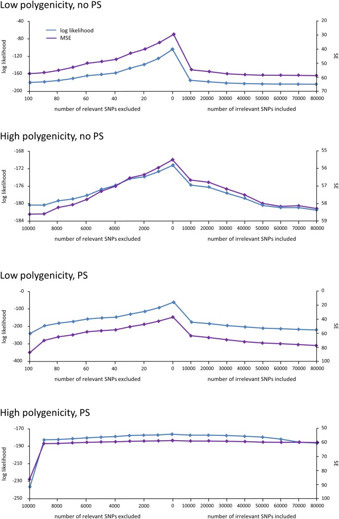
The effects of excluding relevant SNPs and including irrelevant SNPs on phenotype prediction.
Out-of-sample log likelihood  (blue) and squared error (purple) averaged over the folds of cross validation are plotted as a function of the number of relevant SNPs randomly excluded (left) and number of irrelevant SNPs randomly included (right) in the RRM.
To study the effects of variable selection on prediction, we used a simple approach. As discussed in the next section, this approach will also be useful for GWAS. Our approach searched over various sets of SNPs to identify those that maximized cross-validated prediction accuracy. To keep the search practical, we ordered SNPs for each fold by their univariate linear-regression P values on the training data for that fold. We then used increasing numbers of SNPs by this ordering, measuring prediction accuracy on the out-of-sample test set. Next, we averaged the prediction accuracy over each fold. Finally, we identified the number of SNPs k that optimized this average. This method for variable selection (using either the log-likelihood or squared-error criterion) chose 40 for the low and all 80,100 SNPs for the high polygenicity cases, respectively (Figure 2, left column).
Figure 2
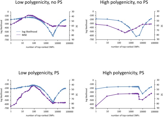
Variable selection for phenotype prediction.
For each fold in 10-fold cross-validation, SNPs are sorted by their univariate P values on the training data. Then, the top k SNPs are used to train the LMM. Finally, the out-of-sample log likelihood  and squared error are computed using the LMM and averaged over the folds. The plots show the averaged log likelihood (blue) and squared error (purple) as a function of k.
We next explored exclusion and inclusion of SNPs on two additional datasets with population structure, roughly emulating what might be found in typical GWAS datasets. For these generated datasets, we used an identical set of SNPs, except that we additionally included a set of either 100 or 10,000 SNPs (for the low and high polygenicity cases, respectively) from two populations, using the Balding-Nichols model20 with a 60:40 population ratio, an F ST = 0.1 and parent population MAFs drawn from a uniform distribution on [0.05, 0.4]. Finally, to inject population structure into the phenotype, we modified the earlier phenotype generation process by adding or subtracting the quantity π to the LMM-generated phenotype variable, depending on the population membership of the individual (as in the Balding-Nichols model). We used  , corresponding to a variance of 0.1 explained by the confounding population variable. Note that, given this generation process, the differentiated SNPs are not causal, but are relevant to the phenotype.
For these two datasets with population structure, we again found that, as the number of (randomly) excluded relevant SNPs or the number of included irrelevant SNPs increased, out-of-sample prediction accuracy decreased substantially (Figure 1). In addition, the simple variable-selection method described previously (using either the log-likelihood or squared-error criterion) chose 125 SNPs and 900 SNPs for the low and high polygenicity case, respectively (Figure 2, right column).
Interestingly, for all four datasets (low and high polygenicity and with or without population structure), predictive accuracy as a function of k, the number of SNPs used to train the LMM, showed a large dip followed by an increase as k was increased (Figure 2). The large dip is due to overfitting of the ratio  , which is fit by an in-sample maximization of the restricted likelihood (i.e., REML). When this ratio is fit with out-of-sample maximization, the magnitude of the dip is greatly decreased. For example, in the high polygenicity dataset with population structure using REML, the prediction accuracy as measured by negative squared error at its maximum (900 SNPs) and local minimum (16,000 SNPs) is −58.9 and −70.5, respectively (Figure 2). In contrast, when this ratio is fit out-of-sample, the negative squared error at 16,000 SNPs is −59.2.
Genome-wide association studies
The next application of LMMs to genomics that we consider is GWAS. LMMs have been used for both univariate6,7,8,9,10,21 and set tests13,14, but here we concentrate on univariate testing for simplicity. In this application, the strength of association between a test SNP and the phenotype is determined with, for example, an F test, wherein the null model is the LMM described above and the alternative model additionally has the test SNP as a fixed effect.
Looking at GWAS from the linear-regression viewpoint, we should use covariates that include causal SNPs, SNPs that tag unavailable causal SNPs and SNPs that are associated with the phenotype via hidden or confounding variables9. The inclusion of causal or tagging SNPs as covariates can improve power by reducing the model misspecification that would otherwise result from their exclusion. (Note that, when there is ascertainment bias, their inclusion can reduce power22. In our experiments, we generate the phenotype without ascertainment bias. For real data, care should be taken.) The inclusion of SNPs that are associated with confounding variables helps to correct for the confounding by effectively conditioning on them. In particular, typically more than one SNP is associated with a confounder. Therefore, when testing such a SNP, there will be another SNP correlated to it that is being used as a covariate, reducing the strength of association of the tested SNP and therefore avoiding a potential false-positive association. Finally, as we have discussed, using SNPs as covariates is equivalent to using them in the RRM with an LMM. Herein, we take this approach.
The extent to which these conditioning effects are beneficial is closely related to the extent to which the RRM contributes to phenotype prediction accuracy. That is, the more predictive these covariates are of the phenotype, the more so conditioning on them yields increased power and less inflation of the test statistic. Consequently, exclusion of relevant SNPs (causal or differentiated) and inclusion of irrelevant SNPs in the RRM, both of which create model misspecification, should diminish the beneficial conditioning effects, thereby leading to a decrease in power and an increase in inflation.
To examine these phenomena empirically, we applied the LMM to the low and high polygenicity datasets with population structure used earlier to study prediction. We computed a P value for the degree of association between each SNP and the phenotype. Then, to assess the effects of exclusion and inclusion of SNPs in the RRM on power, we measured the area under the curve (AUC) of the receiver operator characteristic (ROC) curve. When we measured AUC using every SNP in the dataset (including the 80,000 irrelevant SNPs), the AUC did not vary substantially with exclusion of relevant SNPs or inclusion of the irrelevant SNPs. These 80,000 irrelevant SNPs were randomly distributed in the ranking and weakened the effect of our experimental conditions on AUC. Therefore, we measured AUC using only the causal and differentiated SNPs (omitting the irrelevant SNPs), yielding AUC values that varied significantly. As expected, the exclusion of causal SNPs, the exclusion of differentiated SNPs and the inclusion of irrelevant SNPs, all lead to decreased power (Figure 3a).
Figure 3
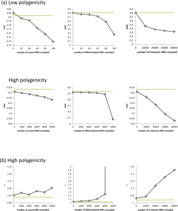
The effects of excluding relevant SNPs and including irrelevant SNPs on power and inflation.
(a) AUC as a function of the number of the causal SNPs excluded (with no irrelevant SNPs included), the number of differentiated SNPs excluded (with no irrelevant SNPs included) and the number of irrelevant SNPs included for the low and high polygenicity cases (including all relevant SNPs). (b) The genomic control factor λ as a function of the number of causal SNPs excluded (with no irrelevant SNPs included), the number of differentiated SNPs excluded (with no irrelevant SNPs included) and the number of irrelevant SNPs included for the high polygenicity case (including all relevant SNPs). The performance of the simple variable-selection method is indicated with green lines. The only plot with a non-monotonic pattern is the one showing λ as a function of the number of causal SNPs excluded (lower left). Nonetheless, the effect is significant in that, with 6,000 or more causal SNPs excluded, the GWAS P value distributions differ significantly from uniform according to a two-sided KS test (P values 0.047, 0.021 and 0.002 for 6,000, 8,000 and 10,000 SNPs excluded, respectively).
To assess the effects of test-statistic inflation from exclusion and inclusion, we measured the genomic control factor,  , for the differentiated SNPs, which are non-causal and should have
  in expectation. Furthermore, we limited our experimental conditions to the high polygenicity dataset, as the low polygenicity dataset contained relatively few differentiated SNPs, leading to high variance estimates of
  . As expected, exclusion of causal SNPs and differentiated SNPs, as well as inclusion of irrelevant SNPs led to inflation (Figure 3b).
Given the connection between prediction and the beneficial condition effects previously discussed, we also expect the LMM to perform well for GWAS when using variable selection. To select SNPs for the RRM, we again identified the number of SNPs k yielding the best out-of-sample predictions as described previously and then selected the k SNPs that had the smallest linear-regression P values on the entire dataset. This selection procedure yielded better power and control for inflation than the use of all SNPs (Figure 3). We also note that, on data from spatially structured populations with rare variants23, this selection procedure yielded similar improvements, in line with earlier results10. Perhaps most interesting, for the high polygenicity dataset, variable selection outperformed the use of precisely all relevant SNPs (Figure 3). That is, excluding some relevant SNPs proved to be beneficial. This result is not surprising as some relevant SNPs will have such a small effect size that they act like irrelevant SNPs, interfering with the proper modelling of the hidden confounder.
Finally, we note that GWAS performance (power and control for inflation) was more sensitive to variable selection than was out-of-sample prediction accuracy. For example, using the high polygenicity dataset with population structure, prediction accuracy with 900 and all 100,000 SNPs was about the same (Figure 2), whereas GWAS performance was quite different (Figure 3). This difference in sensitivity could possibly lead to a situation where, due to a near tie in prediction accuracy for different sets of SNPs, our method would select a set of SNPs with suboptimal GWAS performance. Although we have yet to encounter such a situation in our experiments (including many not reported here), this sensitivity could be mitigated by running GWAS multiple times, each time using the number of ordered SNPs corresponding to one of the near ties in prediction accuracy and then using the analysis that yields the smallest  .
.
Heritability estimation
In this section, we consider the estimation of narrow-sense heritability of a phenotype in a population: the fraction of variance explained by additive genetic effects, excluding effects of dominance and epistasis. We begin with the assumption that the phenotype for individual j, denoted  , is the sum of additive SNP effects:

where  is an offset,
  represents the value of SNP i for individual j,
  is the fixed-effect size relating the value of SNP i to the phenotype and
  is the effect of the environment, assumed to be random with distribution
  . Let
. Let  denote the vector of
  for all individuals j. In contrast to our previous viewpoint, we now consider the
  to be random, such that the collection of
  and
and  are mutually independent and where the distribution of each
  is
is  . Here,
  is the matrix containing the probability of identity by descent between pairs of individuals at each causal variant.
From Equation 2, using the fact that the diagonal entries of  are one, it follows that

Letting  , we then obtain the standard formula for narrow-sense heritability,

Now consider the relationship between Equation 2 and an LMM. Integrating out the  from Equation 2, we obtain

Also, the scatter matrix  , where
  are the observed values of the SNPs, is a consistent estimate for
  . Thus, in this new viewpoint, we return to Equation 1 (with no fixed effects). Consequently, we can apply Equation 1 to estimate
  and
and  and hence
  . We denote such an estimate
  . Finally, note that the two key measures of performance of heritability estimation are the bias and variance of
  .
.
This approach for estimating narrow-sense heritability is different from the more traditional pedigree-based approach24. An advantage of using the LMM over the pedigree-based approach is that we can use SNP data for distantly related individuals, thus mitigating confounding effects from the environment11,12. In fact, when estimating heritability with an LMM, Yang et al.11 advocate the explicit removal of closely related individuals based on the similarity of their SNPs. Also note that using only distantly related individuals mitigates confounding by epistatic and dominance effects12,25.
Because variances are non-negative,  is bounded by 0 and 1. Estimation procedures that enforce these bounds (such as constrained REML) yield biased estimates with lower variance, when compared with unconstrained estimation26. These effects can easily be seen for the case where the true heritability is zero. In this case, for finite data, estimates of heritability will be near zero but always non-negative and hence the expected estimate of heritability will be greater than zero. Similarly, the variance of constrained estimates will be lower than for unconstrained estimates. To quantify this effect, we generated datasets as described above with no population structure, 100 causal SNPs and total variance of 0.2 for 500 individuals. First, we generated 1,000 datasets with a heritability of 0.5, far from the bounds. When using constrained REML, the average difference between
  and
and  was 0.01, well within the standard deviation of
  equal to 0.05, consistent with no bias. Next, we generated 1,000 datasets with a heritability of 0 (on the boundary), yielding an average difference between
  and
and  of 0.015, larger than the standard deviation of
  equal to 0.013, indicating bias and lower variance.
As in the other applications of the LMM, we do not know which SNPs are relevant in practice. Consequently, it is likely that relevant SNPs will be excluded and irrelevant SNPs will be included when performing the estimation. To examine bias and variance due to excluding causal (relevant) SNPs, we used the 1,000 datasets with  described in the previous paragraph, but used 100, 80, 60, 40, 20 and 1 randomly selected SNPs for the RRM. The resulting heritability estimates had averages and standard deviations (in parentheses) of 0.49 (0.05), 0.39 (0.05), 0.29 (0.05), 0.19 (0.05), 0.09 (0.04) and 0.01 (0.02), respectively. Here, there was downward bias from exclusion and a fairly constant level of variance, except for a decrease in variance near the boundary
  . Downward bias with fairly constant variance has been demonstrated previously11.
To examine bias and variance due to including irrelevant SNPs, we report the experiments of Zaitlen and Kraft12, who generated data as we did, except they generated 10 causal SNPs using a MAF range of [0.05,0.5] and a cohort size of 1,500. Adding 100, 1,000 and 5,000 irrelevant SNPs to the RRM, consistently yielded an average  value of 0.50, but the standard deviations were 0.018, 0.025 and 0.067, respectively. The variance increased from inclusion, but bias remained at zero.
In summary, exclusion of relevant SNPs leads to a biased estimate of heritability with little effect on variance, whereas the inclusion of irrelevant SNPs leads to an increase in the variance of the estimate with little effect on bias. These effects are in contrast to the applications of phenotype prediction and GWAS. Roughly, for heritability estimation, exclusion affects bias and inclusion affects variance separately, whereas, in the other applications, exclusion and inclusion both degrade common measures of performance. Consequently, although variable selection is typically useful for phenotype prediction and GWAS, it may not be useful for heritability estimation. For example, when lack of bias is extremely important, variable selection should be avoided. Of course, if one is looking to balance the bias and variance of a heritability estimate, variable selection can still be useful. In this case, variable selection is not simple, because, for a given set of SNPs, one typically obtains a single estimate of  and its variance27. Nonetheless, variable selection could lead to scenarios where the trade-off between bias and variance can reasonably be made. For example, when two sets of variables both yield
  that are relatively close together, but one has much lower estimated variance, then the set of SNPs leading to lower variance may be preferred. In contrast, when two sets of variables both yield
  variances are that relatively close together, but one has much lower
  (due to the downward bias from exclusion), then the set of SNPs leading to higher
  may be preferred.
Set tests
The last use of the mixed model that we examine is determining whether there is a significant association between a phenotype and a set of variants. This task is sometimes referred to as a set test in GWAS13,14. Examples of this task include determining whether a set of rare variants are associated with a phenotype and whether a set of SNPs in a gene or pathway are associated with a phenotype.
As in our discussion of heritability estimation, let us assume that there is no population structure in the data. In this case, to test for association, we build an RRM with the given set of SNPs and test whether  (or equivalently
  ) is greater than zero. As we have seen in the previous section, as the number of relevant SNPs excluded is increased,
  will become increasingly downwardly biased, thereby decreasing the power to detect
  . In addition, as the number of irrelevant SNPs is increased, the variance of
  will increase, thereby again decreasing the power to detect
  . This last effect can be understood by noting that the increased variance in
  arises from a flatter likelihood surface with a lower maximum, which in turn translates to smaller differences between the null and alternative model maximum values of the restricted likelihood.
Often, the set to be tested for association is identified through prior information, leaving no opportunity for variable selection. In some situations, however, there is an opportunity for variable selection. For example, consider the work of Quon et al.28, where they investigated the role played by stretches of _cis_-DNA sequence in influencing human methylation levels for four distinct brain regions, across 150 unrelated individuals. Although they were interested in the influence of _cis_-DNA on methylation loci, they had little prior knowledge on the width of the cis window that contained the bulk of causal SNPs. Consequently, they performed variable selection by way of a window-size selection procedure—considering windows centered on each methylation locus of increasing size. As they increased the window size, the number of loci associated with SNPs first increased and then decreased, yielding a maximum at the window size of 50 kb. This pattern is consistent with our understanding. Namely, the initial increase can be attributed to increasing power due to decreasing downward bias in  and the subsequent decrease can be attributed to decreasing power due to increasing variance in
  .
.
When performing variable selection for set tests, one should be careful to guarantee that the selection criterion and the test statistic ( in our case) are independent under the null hypothesis. For the tests with methylation data, this condition can be achieved by using half of the methylation loci (e.g., on one set of chromosomes) to identify the window size that yields the most associated loci and then applying that window size to the second half of methylation loci. When we applied this procedure to the methylation data processed by Quon et al., we found the window size that maximized the number of identified loci to be the same for the two sets of loci when aggregated across all tissues: 50 kb. When performing the analysis on each brain region separately, among the eight sets tested (four regions for each of the two partitions), there was only one that did not choose 50 kb (Figure 4).
Figure 4
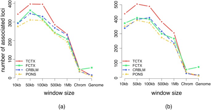
Number of associated methylation loci in the four brain regions (TCTX, FCTX, CRBLM and PONS) that pass a Bonferroni-corrected P value threshold of 0.05 as a function of DNA sequence window size.
Only methylation loci that had at least one SNP in every window were included in the analysis so as to make the windows comparable. The plots are divided into those for even (a) and odd (b) chromosomes.