A map of human genome sequence variation containing 1.42 million single nucleotide polymorphisms (original) (raw)
Main
Inherited differences in DNA sequence contribute to phenotypic variation, influencing an individual's anthropometric characteristics, risk of disease and response to the environment. A central goal of genetics is to pinpoint the DNA variants that contribute most significantly to population variation in each trait. Genome-wide linkage analysis and positional cloning have identified hundreds of genes for human diseases1 (http://ncbi.nlm.nih.gov), but nearly all are rare conditions in which mutation of a single gene is necessary and sufficient to cause disease. For common diseases, genome-wide linkage studies have had limited success, consistent with a more complex genetic architecture. If each locus contributes modestly to disease aetiology, more powerful methods will be required.
One promising approach is systematically to explore the limited set of common gene variants for association with disease2,3,4. In the human population most variant sites are rare, but the small number of common polymorphisms explain the bulk of heterozygosity3 (see also refs 5,6,7,8,9,10,11). Moreover, human genetic diversity appears to be limited not only at the level of individual polymorphisms, but also in the specific combinations of alleles (haplotypes) observed at closely linked sites8,11,12,13,14. As these common variants are responsible for most heterozygosity in the population, it will be important to assess their potential impact on phenotypic trait variation.
If limited haplotype diversity is general, it should be practical to define common haplotypes using a dense set of polymorphic markers, and to evaluate each haplotype for association with disease. Such haplotype-based association studies offer a significant advantage: genomic regions can be tested for association without requiring the discovery of the functional variants. The required density of markers will depend on the complexity of the local haplotype structure, and the distance over which these haplotypes extend, neither of which is yet well defined.
Current estimates (refs 13,14,15,16,17) indicate that a very dense marker map (30,000–1,000,000 variants) would be required to perform haplotype-based association studies. Most human sequence variation is attributable to SNPs, with the rest attributable to insertions or deletions of one or more bases, repeat length polymorphisms and rearrangements. SNPs occur (on average) every 1,000–2,000 bases when two human chromosomes are compared5,6,9,18,19,20, and are thus present at sufficient density for comprehensive haplotype analysis. SNPs are binary, and thus well suited to automated, high-throughput genotyping. Finally, in contrast to more mutable markers, such as microsatellites21, SNPs have a low rate of recurrent mutation, making them stable indicators of human history. We have constructed a SNP map of the human genome with sufficient density to study human haplotype structure, enabling future study of human medical and population genetics.
Identification and characteristics of SNPs
The map contains all SNPs that were publicly available in November 2000. Over 95% were discovered by The SNP Consortium (TSC) and the public Human Genome Project (HGP). TSC contributed 1,023,950 candidate SNPs (http://snp.cshl.org) identified by shotgun sequencing of genomic fragments drawn from a complete (45% of data) or reduced (55% of data) representation of the human genome18,22. Individual contributions were: Whitehead Institute, 589,209 SNPs from 2.57 million (M) passing reads; Sanger Centre, 262,279 SNPs from 1.16M passing reads; Washington University, 172,462 SNPs from 1.69M passing reads. TSC SNPs were discovered using a publicly available panel of 24 ethnically diverse individuals23. Reads were aligned to one another and to the available genome sequence, followed by detection of single base differences using one of two validated algorithms: Polybayes24 and the neighbourhood quality standard (NQS18,22).
An additional 971,077 candidate SNPs were identified as sequence differences in regions of overlap between large-insert clones (bacterial artificial chromosomes (BACs) or P1-derived artificial chromosomes (PACs)) sequenced by the HGP. Two groups (NCBI/Washington University (556,694 SNPs): G.B., P.Y.K. and S.S.; and The Sanger Centre (630,147SNPs): J.C.M. and D.R.B.) independently analysed these overlaps using the two detection algorithms. This approach contributes dense clusters of SNPs throughout the genome. The remaining 5% of SNPs were discovered in gene-based studies, either by automated detection of single base differences in clusters of overlapping expressed sequence tags24,25,26,27,28 or by targeted resequencing efforts (see ftp://ncbi.nlm.nih.gov/snp/human/).
It is critical that candidate SNPs have a high likelihood of representing true polymorphisms when examined in population studies. Although many methods and contributors are represented on the map (see above), most SNPs (> 95%) were contributed by two large-scale efforts that uniformly applied automated methods. Random samples of these SNPs have been evaluated by confirmation in the original DNA samples (where possible) to rule out false positives, and in independent population samples to determine allele frequency. The TSC centres and two outside laboratories (Orchid and Cold Spring Harbor Laboratory) successfully genotyped 1,585 TSC SNPs in the 24 DNA samples used for discovery (http://snp.cshl.org); having surveyed all chromosomes in which each SNP could have been identified, any non-polymorphic candidates must represent false positives. In these tests, 1,500 SNPs (95%) were polymorphic, 67 (4%) non-polymorphic (false positives) and 18 (1%) uniformly heterozygous (previously unrecognized repeats). These high validation rates were observed separately for subsets of SNPs discovered by reduced representation shotgun and genomic alignment, and for subsets identified with Polybayes and the NQS. Thus, these algorithms appear to generate few false positive SNPs. The small number (1%) of uniformly ‘heterozygous’ candidate SNPs show that the methods also exclude nearly all low-copy repeats.
The allele frequencies of a set of SNPs have been evaluated29 in independent populations using pooled resequencing. Samples of TSC (n = 502) and overlap SNPs (n = 774) were studied in population samples of European, African American and Chinese descent, revealing 82% to be polymorphic in at least one ethnic group at frequencies above the detection threshold of pooled resequencing (∼10%). The remaining 18% presumably represent SNPs with a frequency less than 10% in the populations surveyed and false positives. Furthermore, 77% of SNPs had a minor allele frequency of more than 20% in at least one population, and 27% had an allele frequency higher than 20% in all three ethnic groups. TSC and overlap SNPs had similar distributions across the populations, showing that they are comparable in quality and frequency. The high proportion of SNPs with significant population frequency is expected after SNP discovery in two or a few chromosomes, given standard assumptions about human population history18,29,30.
Description of the SNP map
We mapped the sequence flanking each SNP by alignment to the genomic sequence of large-insert clones in Genbank. These alignments were converted into chromosomal coordinates according to the publicly available genome assemblies of July and September 2000 (http://genome.ucsc.edu). Candidate SNPs were included in the final map only if they mapped to a single location in the genome assembly. Integrated displays of SNPs, genes and other features are available at the ENSEMBL (http://www.ensembl.org), NCBI (National Center for Biotechnology Information; http://www.ncbi.nlm.nih.gov), UCSC (University of California at Santa Cruz; http://genome.ucsc.edu) and TSC (http://snp.cshl.org) websites.
The nonredundant SNP total of 1,433,393 is fewer than the sum of individual submissions (2,067,476) because some SNPs (mainly in regions of BAC overlap) were discovered by more than one effort. Of these, 1,419,190 mapped to unique locations in the 2.7 gigabases (Gb) of assembled human genome sequence, providing an average density of one SNP every 1.91 kb. TSC SNPs, which are more evenly distributed than those from clone overlaps, were found on average every 3.05 kb. SNP density (Table 1) is relatively constant across the autosomes. To characterize the distribution of SNPs, we examined 366,192 SNPs that fell within finished sequence. Most of the genome contains SNPs at high density (Fig. 1): 90% of contiguous 20-kb windows contain one or more SNPs, as do 63% of 5-kb windows and 28% of 1-kb windows. Only 4% of genome sequence falls in gaps between SNPs of > 80 kb, and some of these gaps are covered by SNPs that are discovered but not yet mapped owing to gaps in the genome assembly.
Table 1 SNP distribution by chromosome
Figure 1: Distribution of SNP coverage across intervals of finished sequence.
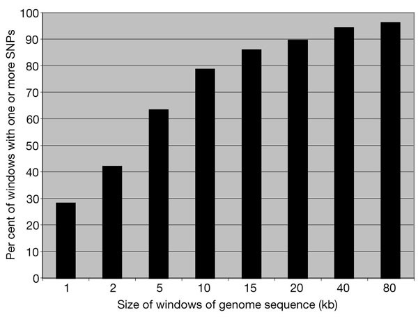
Windows of defined size (in chromosome coordinates) were examined for whether they contained one or more SNPs. Analysis was restricted to the 900 Mb of available finished sequence.
To evaluate the density of SNPs in regions within and surrounding genes, we used the September 2000 release of RefSeq31. In total, 14,534 SNPs map to within these 7,000 carefully annotated, non-redundant messenger RNAs, equivalent to about two exonic SNPs per gene (coding and untranslated regions). Extrapolating two exonic SNPs per gene to the approximately 30,000 human genes32, we estimate there to be 60,000 exonic SNPs in this collection. The density of SNPs in exons (one SNP per 1.08 kb; Table 1) is higher than in the genome as a whole, owing to the contribution of efforts targeted to exonic regions.
We also assessed the distribution of SNPs in the genomic locus surrounding each of the RefSeq mRNAs. We assigned the RefSeq exons to their genomic locations, restricting analysis to the 2,960 RefSeq mRNAs mapping onto finished sequence. As we cannot define the extent of the noncoding (regulatory) regions of each gene, we arbitrarily defined each ‘gene locus’ as extending from 10 kb upstream of the start of the first exon to the end of the last exon. By this definition, 93% of gene loci contain at least one SNP, and 98% are within 5 kb of the nearest SNP; also, 59% of gene loci contained five or more SNPs, and 39% ten or more. Of 24,953 exons, 85% were within 5 kb of the nearest SNP. Thus, most exons should be close enough to at least one SNP for haplotype-based association studies, where the functional variant may be some distance from the SNPs used in the study.
The density of SNPs obtained at any given location depends upon the methods of SNP discovery contributing at each position (TSC, BAC overlap or targeted), the availability of genome sequence for SNP discovery and mapping, and the rate of nucleotide diversity. Of these, only nucleotide diversity is a fundamental characteristic of the region and population studied. To chart the landscape of human genome sequence polymorphism, we performed a genome-wide analysis of nucleotide diversity.
Analysis of nucleotide diversity
Describing the underlying pattern of nucleotide diversity required a polymorphism survey performed at high density, in a single, defined population sample, and analysed with a uniform set of tools. We reanalysed 4.5M passing sequence reads generated by TSC using genomic alignment using the NQS (see Methods). This set contained 1.2 billion aligned bases and 920,752 heterozygous positions. We measured nucleotide sequence variation using the normalized measure of heterozygosity (π), representing the likelihood that a nucleotide position will be heterozygous when compared across two chromosomes selected randomly from a population. π also estimates the population genetic parameter Θ = 4_N_eμ in a model in which sites evolve neutrally, with mutation rate μ, in a constant-sized population of effective size _N_e. For the human genome, π was 7.51 × 10⁻⁴, or one SNP for every 1,331 bp surveyed in two chromosomes drawn from the NIH diversity panel. This value agrees with smaller surveys of human genome variation18,19,20.
We next examined the heterozygosity of individual chromosomes (Table 2). The autosomes were quite similar to one another, with 20 of 22 within 10% of the genome-wide average for autosomes (7.65 × 10⁻⁴). Two had more extreme values: chromosome 21 (π = 5.19 × 10⁻⁴) and chromosome 15 (π = 8.79 × 10⁻⁴). Whether these observations are due to statistical fluctuations or methodological issues, or are biologically meaningful, will require investigation. The most striking difference in heterozygosity is the lower diversity of the sex chromosomes. The lower rate of polymorphism on the X chromosome may be explained by both a lower effective population size (_N_e) and lower mutation rate (μ) in Θ = 4_N_eμ. Because the X chromosome is hemizygous in males, the effective population size is three-quarters of that of the autosomes. In addition, μ is higher in male than in female meiosis, with μmale/μfemale ≈ 1.7/1.0 (ref. 33). As the X chromosome undergoes male meiosis only 1/3 of the time, the overall rate of mutation in the X chromosome is expected to be 91% that of the autosomes (μX = 1.23/1.35 = 0.91). Thus, the diversity of the X chromosome is predicted to be 69% that of the autosomes. The observed heterozygosity of the X chromosome was 4.69 × 10⁻⁴, or 61% of the average value of the autosomes. Thus, the population genetic considerations described above could largely explain the lower heterozygosity on the X chromosome. It is possible that strong selection on the X chromosome (owing to hemizygosity in males) or other factors might partially explain this observation.
Table 2 Nucleotide diversity by chromosome
The Y chromosome has the lowest observed heterozygosity of any chromosome. It is divided into two regions: a pseudoautosomal region at either telomeric end that recombines with the X chromosome and is highly heterozygous34, and the non-recombining Y (NRY). The genome assembly used for this analysis contains only the NRY, which shows very little diversity: 348 SNPs in 2,304,916 bases (π = 1.51 × 10⁻⁴). These values agree reasonably with previous estimates for NRY35,36. The lower diversity of NRY is influenced by a smaller effective population size (20% that of the autosomes), counterbalanced by the higher mutation rate of male meiosis (μY = 1.7/1.35 = 1.26 × that of the autosomes). These factors predict that the Y chromosome would have a diversity 31% that of the autosomes, as compared to the observed 20%. Other influences might include selection against deleterious alleles, patterns of male dispersal35 and a correlation of diversity with recombination rate19.
To look at diversity on a finer scale, we divided each chromosome into contiguous 200,000-bp bins according to the public Genome Assembly of 5 September 2000. The distribution of heterozygosity among these bins ranges from zero (12 bins, each with zero SNPs over an average of 24,720 bp examined) to 60 × 10-4 (357 SNPs in a bin surveying 58,755 bp). Although 95% of bins display nucleotide diversity values between 2.0 × 10⁻⁴ and 15.8 × 10⁻⁴, the pattern is variable (Fig. 2a, b; see also Supplementary Information). One measure of the spread in the data is the coefficient of variation (CV), the ratio of the standard deviation (σ) to the mean (μ) of the heterozygosity π of each individual read. For the observed data, the CV (σobserved/μobserved) was 1.93, considerably larger than would be expected if every base had uniform diversity, corresponding to a Poisson sampling process (σPoisson/μPoisson = 1.73). It was expected that the observed distribution would be much more variable than a Poisson process, because both biochemical and evolutionary forces cause diversity to be nonuniform across the genome. Biological factors may include rates of mutation and recombination at each locus. For example, heterozygosity is correlated with the GC content for each read (Fig. 2c), reflecting, at least in part, the high frequency of CpG to TpG mutations arising from deamination of methylated 5-methylcytosine. Population genetic forces are likely to be even more important: each locus has its own history, with samples at some loci tracing back to a recent common ancestor, and other loci describing more ancient genealogies. The time to the most recent common ancestor at a particular stretch of DNA is variable, and represents the opportunity for sequence divergence; thus, the expected pattern of heterozygosity is more heterogeneous than if every locus shared the same history37,38.
Figure 2: Distribution of heterozygosity.

a, The genome was divided into contiguous bins of 200,000 bp based on chromosome coordinates, and the number of high-quality bases examined and heterozygosity calculated for each. A histogram was generated of the distribution of heterozygosity values across all such bins. b, Heterozygosity was calculated across contiguous 200,000-bp bins on Chromosome 6. The blue lines represent the values within which 95% of regions fall: 2.0 × 10⁻⁴-15.8 × 10⁻⁴. Red, bins falling outside this range. The extended region of unusually high heterozygosity centred at 34 Mb corresponds to the HLA. c, Correlation of nucleotide diversity with GC content of each read (autosomes only). The GC content and heterozygosity of reads from the heterozygosity analysis was calculated after sorting of reads by GC content and separation into 10 bins of equal size. Each bin contains ∼150 Mb of aligned, high-quality sequence.
To assess whether gene history would account for the observed variation in heterozygosity, we compared the observed CV to that expected under a standard coalescent population genetic model. For each read, we adjusted μ on the basis of its per cent GC and length, and simulated genealogical histories under the assumption of a constant-sized population with _N_e = 10,000. The CV determined under this model (σconstant-size/μconstant-size = 1.96) is a close match to the observed data. To estimate standard deviations around these estimates of the CV, it was necessary to consider that tightly linked regions may display correlated histories, and thus are nonindependent. We sampled subsets of the data chosen to minimize correlation among reads (see Methods), providing estimates of the mean and standard deviation of CV for the observed and simulated data (Table 3). These results indicate that the observed pattern of genome-wide heterozygosity is broadly consistent with predictions of this standard population genetic model (for comparison, see an analysis of variation in heterozygosity in the mouse genome)39. However, much work will be required to assess additional factors that could influence this distribution: biological factors such as variation in mutation and recombination rates, historical forces such as bottlenecks40,41, expansions or admixture of differentiated populations, evolutionary selection, and methodological artefacts.
Table 3 Coefficients of variation for the observed data and the Poisson and coalescent models
Regions of low diversity were more prevalent on the sex chromosomes. Whereas only 2.5% of 200,000-bp bins across the genome had π < 2.0 × 10⁻⁴, 15% of bins on the X chromosome42 and 89% on the Y chromosome (NRY) had these levels of diversity. Regions of low diversity may be explained by the smaller effective population size of the sex chromosomes and the variable underlying distribution of heterozygosity. Strong selection acting on the sex chromosomes in males might also have a role, but this hypothesis requires further testing. Regions of high heterozygosity were also observed. One was found on chromosome 6 (Fig. 2b, centred on 34 Mb), and was confirmed to represent the HLA locus, which has high nucleotide diversity owing to balancing selection43. Other regions of varying size were observed on this and other chromosomes (Fig. 2c and Supplementary Information). Some of these highly diverse regions might have also experienced balancing selection, but there are other possible explanations: for example, sampling fluctuations of the coalescent distribution, regions with high rates of mutation and/or recombination, unrecognized duplications in the human genome and sequencing of a rare haplotype by the HGP (to which the TSC reads were compared).
Given the unfinished state of publicly available sequence data and genome assembly, it will be important to reevaluate these estimates as more complete genome sequence becomes available.
Implications for medical and population genetics
We describe a map of publicly available SNPs (as of November 2000), fully integrated with the sequence, physical and genetic maps of the human genome. We anticipate immediate application to studies of human population genetics, candidate-gene studies for disease association, and eventually unbiased, genome-wide association scans. First, the map provides an unprecedented tool for studying the character of human sequence variation. We use these data to describe the first genome-wide view of how human DNA sequence varies in the population, and the public availability of these data should fuel future research into biological and population genetic influences on human genetic diversity.
Second, insights into human evolutionary history will be obtained by using SNPs from the map to characterize haplotype diversity throughout the genome. Human haplotype structure remains largely unexplored, and this map makes it possible to define the extent and variation of haplotype identity, the number and frequencies of common haplotypes, and their distribution among and within existing ethnic groups.
Most practically, where a gene has been implicated in causing disease (by chromosomal position relative to linkage peaks, known biological function or expression pattern), it is desirable exhaustively to survey allelic variation for any association to disease. Using the SNP map, it should be possible to evaluate the extent to which common haplotypes contribute to disease risk. As the speed and efficiency of SNP genotyping increases, such studies will fuel increasingly comprehensive tests of the hypothesis that common variants contribute significantly to the risk of common diseases. To the extent that such studies are successful, they should profoundly affect our understanding of disease, methods of diagnosis, and ultimately the development of new and more effective therapies.
Methods
SNP identification
Candidate SNPs were identified by detection of high-confidence base differences in aligned sequences. For TSC, sequence reads were filtered to exclude low quality reads and those containing predominantly known repetitive sequence. Sequences were aligned to each other using the reduced representation shotgun (RRS) method, and by genomic alignment (GA) as described18,22. For GA of TSC data, reads were compared to available large-insert clones (finished and draft with available PHRAP quality scores) in Genbank. For the analysis of clone overlaps, all available finished and unfinished genomic sequence accessions were aligned. Two methods were used to detect SNPs. The NQS relies upon the sequence trace quality surrounding the SNP base to increase base-calling confidence18,22; most data discovered using the NQS was processed using SsahaSNP, an ultrafast, hash-based implementation of the algorithm (Z.N., A. Cox and J.C.M, manuscript in preparation). The second method calculates confidence scores on the basis of a Bayesian analysis of confidence scores24. A variety of methods were used to find SNPs in expressed sequence tag (EST) overlaps24,25,27 and for targeted resequencing; details of the remaining SNPs can be found in the individual dbSNP entries (http://www.ncbi.nlm.nih.gov/SNP/).
Mapping of SNPs and features
MEGABLAST44 was used to align TSC SNP flanking sequences to the genomic sequence accessions. A SNP was considered mapped if a high-quality match (99% identity or greater) was found across the available flanking sequence of no less than 270 bp. SNPs that matched more than three accessions with identity > 98% were judged to be possible repetitive regions and set aside. SNP coordinates were generated relative to the OO18 build of the genome assembly (5 September 2000) and the OO15 build (15 July 2000), using the AGP format files provided by D. Haussler (http://genome.ucsc.edu).
The NCBI RefSeq mRNA transcripts31 were aligned to the Genome Assembly using the NCBI SPIDEY alignment tool. Alignment required >97% sequence similarity between mRNA and genome sequence; alignments were refined by taking into account the donor/acceptor sites. In cases where CDS annotations were available in the GenBank record, exons of the CDS were aligned within the confines of the mRNA alignment. Regions of known human repeats were annotated directly using RepeatMasker (A. Smit, unpublished).
Nucleotide diversity analysis
To characterize nucleotide diversity, we required a data set in which all data could be analysed both for the number of high-quality bases meeting quality standards for SNP detection, and for the number of SNPs. To ensure homogeneity of analysis, we performed a single analysis of 4.5 million high-quality TSC reads from the Sanger Centre, Washington University in St. Louis and the Whitehead Center for Genome Research. The GC content of these reads was 41%, the same as the genome as a whole32, and the distribution of read GC content across deciles of the genome (sorted by GC content) was within 10% of the expected value for all bins. The read coverage was well distributed: 88% of contiguous 200,000-bp windows contained over 10,000 aligned bases (5%) surveyed for SNPs (see below). Using a single analytic tool (SsahaSNP, an implementation of the NQS; Z.N., A. Cox and J.C.M, in preparation), these reads were aligned to the available genome sequence (finished and draft with quality scores) and the number of high-quality bases (meeting NQS) and SNPs counted. We limited the analysis to SNPs found by genomic alignment so that the cluster depth of each comparison would be exactly two chromosomes. We precisely measured the target size for SNP discovery by counting the number of positions meeting the NQS. This is desirable because alignments contain positions of both high and low quality, but only those meeting the NQS are candidates for SNP discovery. Where a single TSC read aligned to multiple (overlapping) BACs from the HGP, we averaged the number of SNPs and aligned bp for all pairwise alignments of that read; this weighted evenly those reads mapping to a single BAC and those aligning to a region of overlap. Reads representing repeat loci were excluded using validated criteria18,22: alignments of reads to genome were excluded if they were less than 99% identical. The genome was then divided into contiguous bins of 200,000 bp (based on chromosome-relative coordinates). Individual reads were filtered for repeats: any that aligned to more than one bin in the genome assembly were rejected. Finally, heterozygous positions and bases meeting the NQS were counted. As a final filter for regions containing a high proportion of repeats, we reject any bin for which more than 10% of the reads mapping to that bin also mapped to another chromosome. Finally, to avoid statistical fluctuation due to inadequate sampling, we examined only the 88% of bins in which at least 10,000 aligned bases met the NQS and thus could be examined for SNPs.
Coalescent modelling was performed by simulation38, and assumed a constant-sized population of 10,000 individuals and a mutation rate adjusted for each read on the basis of its GC content (Fig. 2c) and length. To assess the standard deviation around this estimate, the simulation was repeated 100 times. For the observed data, calculating a standard deviation around the CV is difficult owing to the correlation of gene history for closely linked sites. In expectation, this correlation should not alter the mean of the observed coefficient of variation, but does influence its variance. To estimate the variance around the CV for the observed data, we selected 100 reduced data sets, each containing one randomly chosen read from each 200,000-bp bin along the autosomes. In using this approach, we assume that these reads, 200,000 bp apart and sampled from unrelated individuals, have independent genealogies. This random sampling procedure was repeated 100 times to estimate the mean and variance of the observed CV.
The data for the heterozygosity analysis, including the coordinates of each bin, the number of bases examined and number of SNPs identified, is available as Supplementary Information.
References
- Collins, F. S. Of needles and haystacks: finding human disease genes by positional cloning. Clin. Res. 39, 615–623 (1991).
CAS PubMed Google Scholar - Collins, F. S., Guyer, M. S. & Charkravarti, A. Variations on a theme: cataloging human DNA sequence variation. Science 278, 1580–1581 (1997).
ADS CAS PubMed Google Scholar - Lander, E. S. The new genomics: global views of biology. Science 274, 536–539 (1996).
ADS CAS PubMed Google Scholar - Risch, N. & Merikangas, K. The future of genetic studies of complex human diseases. Science 273, 1516–1517 (1996).
ADS CAS PubMed Google Scholar - Li, W. H. & Sadler, L. A. Low nucleotide diversity in man. Genetics 129, 513–523 (1991).
CAS PubMed PubMed Central Google Scholar - Cargill, M. et al. Characterization of single-nucleotide polymorphisms in coding regions of human genes [published erratum appears in Nature Genet. 23, 373 (1999)]. Nature Genet. 22, 231–238 (1999).
CAS Google Scholar - Cambien, F. et al. Sequence diversity in 36 candidate genes for cardiovascular disorders. Am. J. Hum. Genet. 65, 183–191 (1999).
CAS PubMed PubMed Central Google Scholar - Fullerton, S. M. et al. Apolipoprotein E variation at the sequence haplotype level: implications for the origin and maintenance of a major human polymorphism. Am. J. Hum. Genet. 67, 881–900 (2000).
CAS PubMed PubMed Central Google Scholar - Halushka, M. K. et al. Patterns of single-nucleotide polymorphisms in candidate genes for blood-pressure homeostasis. Nature Genet. 22, 239–247 (1999).
CAS PubMed Google Scholar - Nickerson, D. A. et al. DNA sequence diversity in a 9.7-kb region of the human lipoprotein lipase gene. Nature Genet. 19, 233–240 (1998).
CAS PubMed Google Scholar - Rieder, M. J., Taylor, S. L., Clark, A. G. & Nickerson, D. A. Sequence variation in the human angiotensin converting enzyme. Nature Genet. 22, 59–62 (1999).
CAS PubMed Google Scholar - Templeton, A. R., Weiss, K. M., Nickerson, D. A., Boerwinkle, E. & Sing, C. F. Cladistic structure within the human lipoprotein lipase gene and its implications for phenotypic association studies. Genetics 156, 1259–1275 (2000).
CAS PubMed PubMed Central Google Scholar - Eaves, I. A. et al. The genetically isolated populations of Finland and sardinia may not be a panacea for linkage disequilibrium mapping of common disease genes. Nature Genet. 25, 320–323 (2000).
CAS PubMed Google Scholar - Taillon-Miller, P. et al. Juxtaposed regions of extensive and minimal linkage disequilibrium in human Xq25 and Xq28. Nature Genet. 25, 324–328 (2000).
CAS PubMed Google Scholar - Kruglyak, L. Prospects for whole-genome linkage disequilibrium mapping of common disease genes. Nature Genet. 22, 139–144 (1999).
CAS PubMed Google Scholar - Collins, A., Lonjou, C. & Morton, N. E. Genetic epidemiology of single-nucleotide polymorphisms. Proc. Natl Acad. Sci. USA 96, 15173–15177 (1999).
ADS CAS PubMed PubMed Central Google Scholar - Reich, D. E. et al. Linkage disequilibrium in the human genome. Nature (submitted).
- Altshuler, D. et al. An SNP map of the human genome generated by reduced representation shotgun sequencing. Nature 407, 513–516 (2000).
ADS CAS PubMed Google Scholar - Nachman, M. W., Bauer, V. L., Crowell, S. L. & Aquadro, C. F. DNA variability and recombination rates at X-linked loci in humans. Genetics 150, 1133–1141 (1998).
CAS PubMed PubMed Central Google Scholar - Wang, D. G. et al. Large-scale identification, mapping, and genotyping of single- nucleotide polymorphisms in the human genome. Science 280, 1077–1082 (1998).
ADS CAS PubMed Google Scholar - Jorde, L. B. Linkage disequilibrium and the search for complex disease genes. Genome Res. 10, 1435–1444 (2000).
CAS PubMed Google Scholar - Mullikin, J. C. et al. An SNP map of human chromosome 22. Nature 407, 516–520 (2000).
ADS CAS PubMed Google Scholar - Collins, F. S., Brooks, L. D. & Chakravarti, A. A DNA polymorphism discovery resource for research on human genetic variation [published erratum appears in Genome Res. 9, 210 (1999)]. Genome Res. 8, 1229–1231 (1998).
CAS Google Scholar - Marth, G. T. et al. A general approach to single-nucleotide polymorphism discovery. Nature Genet. 23, 452–456 (1999).
CAS PubMed Google Scholar - Buetow, K. H., Edmonson, M. N. & Cassidy, A. B. Reliable identification of large numbers of candidate SNPs from public EST data. Nature Genet. 21, 323–325 (1999).
CAS PubMed Google Scholar - Gu, Z., Hillier, L. & Kwok, P. Y. Single nucleotide polymorphism hunting in cyberspace. Hum. Mutat. 12, 221–225 (1998).
CAS PubMed Google Scholar - Irizarry, K. et al. Genome-wide analysis of single-nucleotide polymorphisms in human expressed sequences. Nature Genet. 26, 233–236 (2000).
CAS PubMed Google Scholar - Picoult-Newberg, L. et al. Mining SNPs from EST databases. Genome Res. 9, 167–174 (1999).
CAS PubMed PubMed Central Google Scholar - Marth, G. T. et al. Single nucleotide polymorphisms in the public database: how useful are they? Nature Genet. (submitted).
- Yang, Z. et al. Sampling SNPs. Nature Genet. 26, 13–14 (2000).
CAS PubMed Google Scholar - Pruitt, K. D., Katz, K. S., Sicotte, H. & Maglott, D. R. Introducing RefSeq and LocusLink: curated human genome resources at the NCBI. Trends Genet. 16, 44–47 (2000).
CAS PubMed Google Scholar - International Human Genome Sequencing Consortium. Initial sequencing and analysis of the human genome. Nature 409, 860–921 (2001).
ADS Google Scholar - Bohossian, H. B., Skaletsky, H. & Page, D. C. Unexpectedly similar rates of nucleotide substitution found in male and female hominids. Nature 406, 622–625 (2000).
ADS CAS PubMed Google Scholar - Cooke, H. J., Brown, W. R. & Rappold, G. A. Hypervariable telomeric sequences from the human sex chromosomes are pseudoautosomal. Nature 317, 687–692 (1985).
ADS CAS PubMed Google Scholar - Shen, P. et al. Population genetic implications from sequence variation in four Y chromosome genes. Proc. Natl Acad. Sci. USA 97, 7354–7359 (2000).
ADS CAS PubMed PubMed Central Google Scholar - Underhill, P. A. et al. Detection of numerous Y chromosome biallelic polymorphisms by denaturing high-performance liquid chromatography. Genome Res. 7, 996–1005 (1997).
CAS PubMed PubMed Central Google Scholar - Tajima, F. Evolutionary relationship of DNA sequences in finite populations. Genetics 105, 437–460 (1983).
CAS PubMed PubMed Central Google Scholar - Hudson, R. R. in Oxford Surveys in Evolutionary Biology (eds Futuyma, D. & Antonovics, J.) 1–44 (Oxford Univ. Press, Oxford, 1991).
Google Scholar - Lindblad-Toh, K. et al. Large-scale discovery and genotyping of single-nucleotide polymorphisms in the mouse. Nature Genet. 24, 381–386 (2000).
CAS PubMed Google Scholar - Kimmel, M. et al. Signatures of population expansion in microsatellite repeat data. Genetics 148, 1921–1930 (1998).
CAS PubMed PubMed Central Google Scholar - Reich, D. E. & Goldstein, D. B. Genetic evidence for a Paleolithic human population expansion in Africa [published erratum appears in Proc. Natl Acad. Sci. USA 95, 11026 (1998)]. Proc. Natl Acad. Sci. USA 95, 8119–8123 (1998).
CAS Google Scholar - Miller, R. D., Taillon-Miller, P. & Kwok, P. Y. Regions of low single-nucleotide polymorphism (SNP) incidence in human and orangutan Xq: deserts and recent coalescences. Genomics (in the press).
- Horton, R. et al. Large-scale sequence comparisons reveal unusually high levels of variation in the HLA-DQB1 locus in the class II region of the human MHC. J. Mol. Biol. 282, 71–97 (1998).
CAS PubMed Google Scholar - Zhang, Z., Schwartz, S., Wagner, L. & Miller, W. A greedy algorithm for aligning DNA sequences. J. Comput. Biol. 7, 203–214 (2000).
CAS PubMed Google Scholar
Acknowledgements
The SNP Consortium, the Wellcome Trust and the National Human Genome Research Institute funded SNP discovery and data management at Cold Spring Harbor Laboratories, The Sanger Centre, Washington University in St. Louis, and the Whitehead/MIT Center for Genome Research. Work in P.Y.K.'s laboratory is supported in part by grants from the SNP Consortium and the National Human Genome Research Institute. P.Y.K. thanks Q. Li, M. Minton, R. Donaldson and S. Duan for technical assistance. D.M.A. was supported during a phase of this work under a Postdoctoral Fellowship for Physicians from the Howard Hughes Medical Institute. For full list of contributors to TSC programme, see http://www.snp.cshl.org.
Author information
Authors and Affiliations
- Cold Spring Harbor, 11724, New York, USA
Ravi Sachidanandam, David Weissman, Steven C. Schmidt, Jerzy M. Kakol & Lincoln D. Stein - Building 38A, 8600 Rockville Pike, Bethesda, 20894, Maryland, USA
Gabor Marth & Steve Sherry - Wellcome Trust Genome Campus, Hinxton, CB10 1SA, Cambridge, UK
James C. Mullikin, Beverley J. Mortimore, David L. Willey, Sarah E. Hunt, Charlotte G. Cole, Penny C. Coggill, Catherine M. Rice, Zemin Ning, Jane Rogers & David R. Bentley - 660 S. Euclid Ave, St. Louis, 63110, Missouri, USA
Pui-Yan Kwok, Elaine R. Mardis, Raymond T. Yeh, Brian Schultz, Lisa Cook, Ruth Davenport, Michael Dante, Lucinda Fulton, LaDeana Hillier, Robert H. Waterston & John D. McPherson - 9 Cambridge Center, Cambridge, 02139, Massachusetts, USA
Brian Gilman, Stephen Schaffner, William J. Van Etten, David Reich, John Higgins, Mark J. Daly, Brendan Blumenstiel, Jennifer Baldwin, Nicole Stange-Thomann, Michael C. Zody, Lauren Linton, Eric S. Lander & David Altshuler - Department of Biology, Massachusetts Institute of Technology, Cambridge, 02142, Massachusetts, USA
Eric S. Lander - Departments of Genetics and Medicine, Harvard Medical School,
David Altshuler - Department of Molecular Biology and Diabetes Unit, Massachusetts General Hospital, Boston, 02114, Massachusetts, USA
David Altshuler
Consortia
The International SNP Map Working Group
Cold Spring Harbor Laboratories:
- Ravi Sachidanandam
- , David Weissman
- , Steven C. Schmidt
- , Jerzy M. Kakol
- & Lincoln D. Stein
National Center for Biotechnology Information:
- Gabor Marth
- & Steve Sherry
The Sanger Centre:
- James C. Mullikin
- , Beverley J. Mortimore
- , David L. Willey
- , Sarah E. Hunt
- , Charlotte G. Cole
- , Penny C. Coggill
- , Catherine M. Rice
- , Zemin Ning
- , Jane Rogers
- & David R. Bentley
Washington University in St. Louis:
- Pui-Yan Kwok
- , Elaine R. Mardis
- , Raymond T. Yeh
- , Brian Schultz
- , Lisa Cook
- , Ruth Davenport
- , Michael Dante
- , Lucinda Fulton
- , LaDeana Hillier
- , Robert H. Waterston
- & John D. McPherson
Whitehead/MIT Center for Genome Research:
- Brian Gilman
- , Stephen Schaffner
- , William J. Van Etten
- , David Reich
- , John Higgins
- , Mark J. Daly
- , Brendan Blumenstiel
- , Jennifer Baldwin
- , Nicole Stange-Thomann
- , Michael C. Zody
- , Lauren Linton
- , Eric S. Lander
- & David Altshuler
Corresponding authors
Correspondence toDavid R. Bentley or David Altshuler.
Additional information
(contributing institutions are listed alphabetically).
Rights and permissions
About this article
Cite this article
The International SNP Map Working Group. A map of human genome sequence variation containing 1.42 million single nucleotide polymorphisms.Nature 409, 928–933 (2001). https://doi.org/10.1038/35057149
- Received: 28 November 2000
- Accepted: 27 December 2000
- Issue Date: 15 February 2001
- DOI: https://doi.org/10.1038/35057149