Half of the world’s population experience robust changes in the water cycle for a 2 °C warmer world (original) (raw)
1748-9326/9/4/044008
Abstract
Fresh water is a critical resource on Earth, yet projections of changes in the water cycle resulting from anthropogenic warming are challenging. It is important to not only know the best estimate of change, but also how robust these projections are, where changes occur, which variables will change, and how many people are affected by it. Here we synthesize the changes in the water cycle, based on results of the latest climate model intercomparison (CMIP5). Several variables of the water cycle, such as evaporation and relative humidity, show robust changes over more than 50% of the land area already with an anthropogenic global warming of 1 °C. A warming of 2 °C shows more than half of the world’s population to be directly affected by robust local changes in the water cycle, and everybody experiences a robust change in at least one variable of the water cycle. While the physical changes are widespread, the affected people are concentrated in a few hot-spots mainly in Asia and Central Africa. The occurrence of these hot-spots is driven by population density, as well as by the early emergence of the anthropogenic signal from variability in these areas. Large uncertainties remain in projections of soil moisture and runoff changes.
Export citation and abstractBibTeXRIS
Water is one of the most valuable resources on Earth. Our life, the ecosystems and the services they provide, energy production from hydropower, agriculture and food production, snow and glaciers for tourism, they all heavily rely on water resources. Through latent heat the water cycle is also a critical component of the energy budget, and therefore modifies temperature. The United Nations World Water Development Report 4 (WWAP (World Water Assessment Programme), 2012) concluded that water is the only medium with which global crises such as food, energy, and health can be addressed jointly. Thus the knowledge of projected changes in the water cycle is decisive for impacts, mitigation and adaptation strategies. At the same time, the water cycle is complex and changes in many aspects are still uncertain despite models describing more of the relevant processes in greater detail.
A number of studies have produced indices aggregating various aspects of climate change, e.g. temperature, precipitation, and/or extremes, and have identified ‘hot-spots’, i.e., areas where changes are most pronounced (Giorgi 2006, Baettig et al 2007, Diffenbaugh and Giorgi 2012). Others have identified regions in which the climate change signal will first emerge from natural variability (Williams et al 2007, Scherrer and Baettig 2008, Battisti and Naylor 2009, Giorgi and Bi 2009, Diffenbaugh and Scherer 2011, Hawkins and Sutton 2011, Mahlstein et al 2011, Deser et al 2012a, Mahlstein et al 2012). Almost all studies have assessed the multi-model mean change relative to either internal climate variability or to model spread, but have not considered both simultaneously. Often studies have set the criteria for an emerging signal as a fraction of models showing significant change, without considering the model agreement on the magnitude of change. Natural variability at individual locations and for trends over less than a few decades is large, in particular for precipitation and other aspects of the water cycle (Deser et al 2012a, 2012b, Mahlstein et al 2012). The forced climate change signal can be used to describe changes resulting from anthropogenic influence (e.g. by averaging many simulations). However, when making a statement about future changes in the single realization of the real world and at a particular location, then natural variability must be considered. Model agreement should also be considered, but is only relevant if changes are significant with respect to internal variability; if the changes are within variability, there is no reason for models to agree on the sign of change (i.e., Tebaldi et al 2011, Power et al 2012). Here we build on an earlier study (Knutti and Sedláček 2012) where we introduced a robustness measure which considers the magnitude of change, the internal variability, and the model agreement in a comprehensive and quantitative way.
The impacts of changes in the water cycle on human health, infrastructure, agriculture, tourism etc are complex and diverse, and aggregating their overall effect is far beyond the scope of this manuscript. For some plants, for example, a tendency towards wetter conditions will be favorable, whereas for others it will be harmful. Impacts depend on the region, the season, the magnitude, and the sector. Here we investigate the changes in the water cycle from the point of view of their robustness in the physical changes, and link them to the population living in a particular place. This essentially shows which aspects of the water cycle will change, where, how much, whether those changes are significant relative to natural variability, how well models agree in projecting those, and how many people are living there that might potentially experience it or be directly affected by it.
The most relevant hydrological fields for people, i.e., precipitation, evaporation, relative humidity, soil moisture and runoff, used in this study are taken from 15 models participating in the fifth phase of the Coupled Model Intercomparison Project CMIP5 (Taylor et al 2011). The number of models is determined by the availability of the fields of interest. For consistency across variables, only models that provide all fields are considered. Anomalies are calculated for 20-year periods relative to the 1981–2005 climatology. The Representative Concentration Pathway RCP 8.5 is used as a scenario for the projected future changes (Meinshausen et al 2011). Although the magnitudes are different, patterns of change will be similar for many other scenarios and can be scaled (Tebaldi and Arblaster 2014). The impact and changes are calculated for two ‘seasons’, i.e., April–September and October–March. Changes in water cycle related extremes are not considered here and changes in snow and ice neither.
Two quantities are used to assess the model results, the robustness and the significance. The ‘robustness’ was introduced by Knutti and Sedláček (2012) and is adapted from the ranked probability skill score used in numerical weather predictions (Weigel et al 2007). It is a measure of how the projections from the different models agree on the sign and magnitude of change, including the shape of the distribution and its variability. A value of one denotes high robustness (perfect agreement across models) while low values (zero or below) indicate poor agreement. In this study we use 0.8 as a threshold for a robust change. Details about the method are discussed in Knutti and Sedláček (2012). The significance, i.e., the number of models showing significant mean changes relative to the base period using a _t_-test with a 95% confidence, is also computed. If more than 80% of the models show no significant change then we label this as non-significant. The two measures are independent, and there can be regions where the changes are robust but non-significant (models agreeing on a change in variability with little change in mean, although that case is rare) or significant but not robust (models indicating strong change but disagreeing in sign or magnitude). Following Collins et al (2013, Box 12.1) we show changes for the multi-model mean in all locations and stipple areas with robust changes (i.e., most models indicating changes and agreeing well on magnitude and sign), and hatch areas with no significant change (i.e., at least 80% of the models showing no significant change).
In general, significance of changes and robustness across models are determined by the agreement of models on the forced response, and the magnitude of the response compared to internal variability. A robust response in our results (stippling) requires that the changes are different from present day variability and models agree on the magnitude of change (Knutti and Sedláček 2012).
The projected changes in population used in this study are taken from estimates of population change from the GGI Scenario Database developed at the International Institute for Applied System Analysis (IIASA) (Riahi and Nakicenovic 2007). The population growth is computed to be consistent with the Special Report on Emission Scenarios SRES A2, which is similar to RCP8.5 in terms of climate change (Knutti and Sedláček 2012). The estimated total population roughly doubles from 6.0 billions in year 2000 to 12.4 billions in 2100. The main conclusions (in terms of fraction of populations) are not sensitive to the choice of the population projections, but the absolute number of people is.
All models are treated equally here. Some models perform better than others compared to present day climate and some models are near-duplicates in CMIP5 (Knutti et al 2013), but constraints of present day climate on projections are weak and only looking at a specific subset of models does not significantly change the robustness (Knutti et al 2010, Scherrer 2011, Knutti and Sedláček 2012). Formal methods to consider model performance and model interdependence are in their infancy, and thus not an option for this analysis.
We look at the changes in key variables of the hydrological cycle at the end of the century: precipitation (P), evaporation (E), P–E, relative humidity, soil moisture, and runoff (see figures 1 and 2 for the two different seasons). This study focuses on the regional emerging changes of the hydrological cycle and we provide only a brief discussion on the large-scale mechanisms. An in-depth discussion of future changes in the water cycle, including the relevant mechanisms, is given by Collins et al (2013).
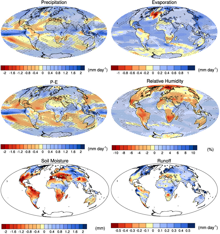
Figure 1. Changes in the Northern Hemisphere winter (October–March) water cycle projected for the end of the century in the RCP8.5 scenario (2081–2100 minus 1896–2005). Dots denote regions where the changes are robust and the hatching represents regions where the changes are not significant relative to internal climate variability.
Download figure:
Standard imageHigh-resolution image
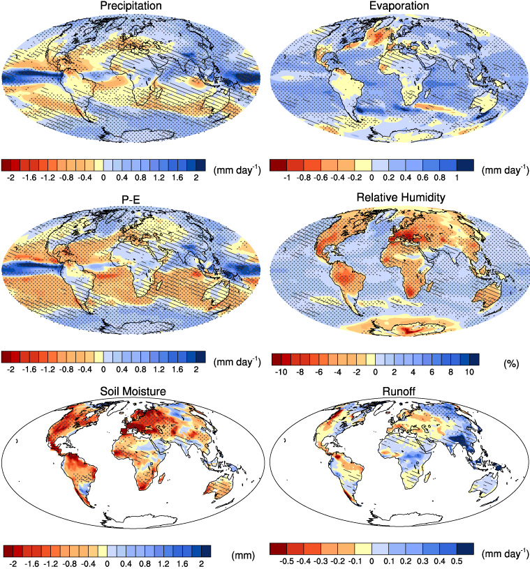
Figure 2. As figure 1 but for April–September.
Download figure:
Standard imageHigh-resolution image
Over large parts of the globe the projections are similar for both seasons (figure 1 versus 2). Each of the key variables we select is of importance to the local experience of the water cycle. However, they are also intricately linked through local, regional, and global phenomena. The links between changes can be briefly summarized as follows: as a result of higher temperatures, the atmosphere is able to store more water vapor in absolute terms. Global relative humidity stays approximately constant, but increases over the oceans and decreases over land as a result of stronger warming over land and limited soil moisture availability for evapotranspiration. Increased water vapor in the atmosphere increases moisture convergence in the tropics and moisture divergence at the descending branch of the Hadley circulation. Thus precipitation increases over the tropics and decreases over the mid-latitudes (e.g., Held and Soden 2006). At high latitudes, precipitation increases robustly as a result of warmer air holding and transporting more water. Global mean precipitation increases by 1–3% °C−1, much less than the change in saturation water vapor pressure (Allen and Ingram 2002). In addition to the thermodynamic response, there will very likely be changes in the atmospheric circulation (Marvel and Bonfils 2013), e.g., a poleward shift in the storm tracks, and a weakening and widening of the Hadley cell, the latter partially offsetting the intensification of the hydrological cycle due to increased temperatures. Warming and the direct effects of CO2 on the atmospheric circulation dominate precipitation changes, for example, through changes in the lapse rate. However, other radiative forcings can be important at the regional scale.
The increased temperatures enhance evaporation over most of the globe. As a consequence, soil moisture is reduced as the availability of stored water is limited and hence the relative humidity over land is also reduced. Over the ocean on the other hand, water availability is not limited and the relative humidity is increased. The regional changes of runoff in the long term follow the availability of water on the surface, i.e., P–E (precipitation minus evaporation).
From figures 1 and 2 it is also evident that the variables that respond fast to changes in temperature such as precipitation, evaporation and relative humidity are robust over almost the entire globe at the end of the century. Soil moisture and runoff are only indirectly related to temperature. For example, plants will use part of the water, or parts of the land area will be frozen. In addition, processes related to hydrology, soils and vegetation are complex, small-scale, are often poorly represented in climate models, and observations to evaluate models are sparse and uncertain (Seneviratne et al 2010). All of these factors result in a smaller area of robust soil moisture and runoff changes. The few robust changes are a drying in some already dry areas and an increase in high latitude runoff.
At a global mean temperature increase of 1 °C from present climate (1986–2005), evaporation (E) and relative humidity experience robust changes over 50% of the land area, as shown in figure 3. However, about 50% or more of the area still shows changes that are non-significant. Precipitation (P) and P–E have slightly lower area fractions which are robust and well over 50% of the area where changes are non-significant. Soil moisture and runoff have only small areas that are robust. Note that Antarctica and Greenland do not have values for soil moisture and runoff, thus the potential possible coverage is slightly lower than 1. Anomalies are calculated from the 1986 to 2005 average here, but as a result of pattern scaling the same conclusions hold for warming relative to preindustrial.
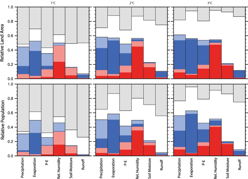
Figure 3. Relative fraction of land (top) and population (bottom) that are projected to experience robust (both light and dark red/blue) and non-significant (gray and light colors) for a change of global mean temperature of 1–3 °C. Dark colors are fractions where the changes are robust and light colors denote changes that are robust but non-significant. Red indicates negative changes and blue positive changes. Gray represents fraction that are non-significant and not robust.
Download figure:
Standard imageHigh-resolution image
A further increase in global temperature to 2 °C will increase the land fraction that shows robust changes and decrease the non-significant areas. This is best visible for precipitation and evaporation. Interestingly, the decrease of non-significant areas is not compensated by robust areas but rather by an increase in areas with uncertain changes, i.e. places where more than 20% of the models show significant change and the robustness is less than 0.8 (the regions in figures 1 and 2 without stippling and hatching, indicated as white bars in figure 3).
For a temperature change of 3 °C from today’s levels, over 50% of the land area is affected by robust changes in precipitation, evaporation, P–E and relative humidity. As before, there is again a large decrease in non-significant areas and modest additional regions with robust changes. Knutti and Sedláček (2012) showed that the land area fraction that shows robust changes in temperature and precipitation increases rapidly for small temperature changes, as a result of the climate change signal emerging from variability. It then reaches nearly constant values as global temperature increases further because model disagreement on the magnitude of change becomes important. The non-significant areas on the other hand converge to near zero with increasing temperature change independently of the variable. This behavior of robustness and non-significant change is inherent to the system and is present in all variables, but happening more or less quickly for the different variables as the climate change emerges. For example, the robustness in P–E increases more quickly than that of soil moisture. It would qualitatively be similar even if model uncertainty were eliminated (Knutti and Sedláček 2012). The results here are broadly consistent with recent studies highlighting water scarcity in large regions for a warming of 2–3 °C (Gerten et al 2013, Schewe et al 2013), but also highlight important remaining uncertainties in our ability to represent soil processes and hydrology in global models (Seneviratne et al 2010, Dadson et al 2013).
The population whose environment is directly affected by the local change of the hydrological cycle follows a similar path as the land area affected (figure 3, second row), but there are a few noticeable differences. The initial increase in population which experience robust direct changes with increasing temperature is larger compared to the change of robustness of the land area. At low magnitudes of climate change, the regions where the robust changes occur are mostly areas where population is low (with the exception of Europe and parts of North America, see figure 4). As the temperature increases, more areas that are located in Asia, Africa and Australia show robust changes, leading to higher fractions of population affected (see also figure 4). The opposite is true for the non-significant areas. For small temperature change the regions with high population density show non-significant changes while at higher temperature the non-significant areas shift to less populated regions.
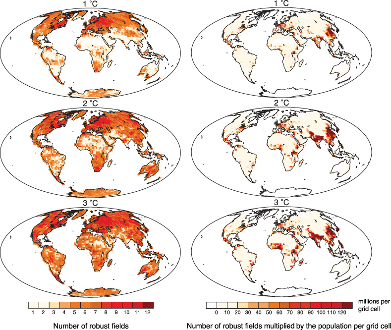
Figure 4. Left: number of robust fields (out of 12) with robust changes for three different global mean temperature changes. Right: number of robust fields multiplied by the population per grid cell. Red colors imply large population density as well as robust changes in many fields.
Download figure:
Standard imageHigh-resolution image
For an additional temperature change of 2 °C, which corresponds roughly to the warming projected at mid-century in a high emission scenario, already half of the population experience robust changes in precipitation and relative humidity. At the end of the century, when mean temperature increase exceeds 3 °C in RCP8.5, more than half of the world’s population is robustly affected by changes in precipitation, evaporation and relative humidity. Robust changes in P–E affect slightly less than 50% of the population. About 10–20% of the population will be affected by changes in soil moisture and runoff. For these two variables the robustly affected areas are smaller and thus the potential to affect a large population is also smaller. In the case of runoff, most changes occur in the high latitudes where population is low (figures 1 and 2).
Note that population is also changing over time (and thus with temperature). Keeping the population constant yields a slightly larger fraction of the population affected by robust changes, indicating that the population growth in the ‘robust’ areas is slightly smaller than the global population increase. Qualitative results, however, are similar when assuming constant population over time.
The regional distribution of the robust fields is quite different depending on the variable. One question of interest could therefore be: how many people are directly affected by at least one robust field, and how many by at least half of the fields? Already for 1 °C (always relative to 1986–2005), 91% of the world’s population are affected by at least one robust change. For 2 °C and 3 °C, 98% and 100% are affected by at least one field, respectively. About 14%, 42% and 58% will experience robust changes in at least half of the fields for 1 °C, 2 °C and 3 °C, respectively. Keeping the population constant results in very similar numbers. To make the results more useful for a wide range of scenarios, we express changes here as function of warming rather than time. In addition, estimating a particular year in the future where the climate will be different from today is potentially misleading given that several aspects of the trend in the water cycle have already been detected and attributed to human influence (Zhang et al 2007, Min et al 2008, Marvel and Bonfils 2013, Fischer and Knutti 2014). The fraction of people experiencing change will be higher than indicated here because estimating robustness on the map requires models to agree on single grid points. Recent studies showed that there are detectable changes once changes are spatially aggregated even if local changes are not significant in most places (Fischer et al 2013, Fischer and Knutti 2014). In other words, this analysis counts only those areas and people where we can quantify changes with high confidence. As a result of natural variability, there will be places where changes are significant, but we cannot project where these are.
A further question we want to investigate is the geographical distribution of robust changes aggregated over variables and seasons, and the population affected by it. The left column of figure 4 shows the fraction of robust fields (out of the twelve fields—six variables, two seasons—in figures 1 and 2) for an additional warming of 1, 2 and 3 °C, respectively. The right column of figure 4 shows the same quantity multiplied by population density. Nearly white areas denote regions where either no variable shows robust changes or where the population density is very low. A change in color indicates either an increase in population or an additional field that becomes robust. A more in-depth look shows that the latter dominates the picture. Note that due to the averaging over a 20-yr time period delayed effects such as snow storage or soil moisture–river discharge relations are also partly visible.
Already for an additional global temperature increase of 1 °C, people living in large parts of North America, Europe, Siberia, the Amazonian region and South Africa are affected by robust changes in more than 5 fields of the hydrological cycle. For a temperature increase of about 2 °C, the large populations in Southeast Asia and India are additionally affected. Furthermore, people living in northern Africa, Australia and South America begin additionally to experience robust changes directly. Finally, with a temperature change of about 3 °C above present, which corresponds roughly the projected temperature at the end of the century using RCP 8.5, the most substantial changes are in India and Central Africa.
Changes in the water cycle affect people globally. The physical changes are very widespread, but the directly affected people are concentrated in a few hot-spots mainly in India, China and Central Africa. Because our analysis focuses on the share of population that directly experiences robust water cycle changes, it is most likely an underestimate of the total population share affected. Through economic connections, changes in the water cycle in scarcely populated areas can still impact population elsewhere. For example, large areas in Russia, the Ukraine, and the US, are wheat producing regions of global importance. Local shifts of the hydrological cycle in these scarcely populated areas could affect the crop yield and therewith have an impact on population elsewhere. This suggests that our results provide lower-end estimates. An in-depth analysis of such connections, however, lies outside the scope of this paper. Already a temperature increase of 1 °C shows that at least 91% of the population are directly affected by at least one robust change in a field. A temperature increase of 2 °C reduces the non-significant areas and increases the robust areas resulting in more than half of the population affected by robust changes in precipitation, evaporation and relative humidity. Further warming increases the robustness in the areas where changes are already clear, but does not strongly affect the fraction of land or people directly affected. The most robust changes are an increase in precipitation in mid to high latitudes, an increase in evaporation and a decrease of relative humidity over land. Uncertainties are largest and models are least consistent in projections of soil moisture and runoff. Even though uncertainties in projections have not changed much over the last two model intercomparisons (Knutti and Sedláček 2012), we show that even a modest additional global temperature change of 1–2 °C will result in a large fraction of the inhabited land and population to experience changes in one or more variables of the water cycle that are projected to be significant relative to natural variability and consistent in sign and magnitude across a wide range of climate models.
We acknowledge the World Climate Research Programme’s Working Group on Coupled Modelling, which is responsible for CMIP, and we thank the climate modeling groups for producing and making available their model output. For CMIP the US Department of Energy’s Program for Climate Model Diagnosis and Intercomparison provides coordinating support and led development of software infrastructure in partnership with the Global Organization for Earth System Science Portals.