REDSHIFT EVOLUTION IN BLACK HOLE–BULGE RELATIONS: TESTING C iv-BASED BLACK HOLE MASSES (original) (raw)
0004-637X/709/2/937
ABSTRACT
We re-examine claims for redshift evolution in black hole–bulge scaling relations based on lensed quasars. In particular, we refine the black hole (BH) mass estimates using measurements of Balmer lines from near-infrared spectroscopy obtained with Triplespec at Apache Point Observatory. In support of previous work, we find a large scatter between Balmer and UV line widths, both Mg iiλλ2796, 2803 and C ivλλ1548, 1550. There is tentative evidence that C iii]λ1909, despite being a blend of multiple transitions, may correlate well with Mg ii, although a larger sample is needed for a real calibration. Most importantly, we find no systematic changes in the estimated BH masses for the lensed sample based on Balmer lines, providing additional support to the interpretation that black holes were overly massive compared to their host galaxies at high redshift.
Export citation and abstractBibTeXRIS
Locally, we observe tight correlations between the properties of bulge-dominated galaxies and the masses of their central supermassive black holes (BHs; e.g., Kormendy & Richstone 1995; Tremaine et al. 2002; Gültekin et al. 2009). The mechanisms that establish and maintain these relations are uncertain, despite innumerable suggestions in the literature (e.g., Silk & Rees 1998; Murray et al. 2005; Miralda-Escudé & Kollmeier 2005; Hopkins et al. 2006; Peng 2007). In principle, evaluating the demographics of nuclear BHs as a function of redshift should observationally constrain the processes that lead to the tight scaling relations observed today. Unfortunately, it is currently prohibitive to obtain dynamical BH masses for systems beyond tens of Mpc. Thus, estimates of BH mass at large distance are necessarily based on very indirect methods linked to accretion processes in active BHs (e.g., Vestergaard 2002).
Several studies have used active galaxies to probe evolution in BH–bulge scaling relations, probing redshifts from 0.4 < _z_ < 0.6 (Woo et al. 2006; Treu et al. 2007; Woo et al. 2008) and 1 ≲_z_≲ 4 (Peng et al. 2006a, 2006b; Salviander et al. 2007; Shields et al. 2006; Ho 2007; Jahnke et al. 2009; McLeod & Bechtold 2009) all the way to _z_ = 6.4 (Walter et al. 2004). Generally speaking, a wide variety of observations suggest that BH–bulge relations do evolve with redshift, in the sense that the ratio of BH to bulge mass was higher at early times (but see also Shields et al. 2003; Alexander et al. 2008), although we have observational constraints only for the most massive systems (_M_BH >108 _M_☉) at high redshift. This counterintuitive result has stimulated vigorous discussion both about the ramifications for the co-evolution of BHs and bulges (e.g., Robertson et al. 2006; Croton 2006) and about whether there are built-in biases in the measurement techniques (Lauer et al. 2007).
Unfortunately, even apart from potential population biases, our interpretation of the observations is prone to significant uncertainty. On the one hand, it is only possible to obtain BH mass estimates at cosmological distances using active galaxies (typically luminous quasars at high redshift). Immediately, it becomes very challenging to characterize the host galaxy properties, when the quasar outshines the underlying galaxy starlight by factors of ∼10–30 (e.g., Peng et al. 2006a; Kim et al. 2008a). Apart from direct imaging, some groups have used gas measurements (predominantly CO) to obtain dynamical masses (Shields et al. 2006; Ho et al. 2008; Walter et al. 2004; Riechers et al. 2008, 2009), which may or may not provide a reliable tracer of the galaxy mass (Ho 2007). The width of narrow emission lines, particularly [O iii]λ5007, has also been substituted for the galaxy velocity dispersion (e.g., Shields et al. 2003; Boroson 2003; Salviander et al. 2007; Gaskell 2009). While there is a strong correlation between stellar and gaseous velocity dispersion in low-luminosity sources (e.g., Heckman et al. 1981; Nelson & Whittle 1996; Greene & Ho 2005a; Ho 2009), there is good reason to suspect that it does not hold at high luminosity (e.g., Greene et al. 2009). Peng et al. (2006b, P06 hereafter) mitigated the host galaxy contrast problem by focusing on lensed quasars. The quasars are lensed differently from the underlying (resolved) host galaxies, reducing the contrast problem discussed above. For that reason, we focus on the lensed quasar sample in this paper.
Daunting as measuring high-redshift galaxy mass and stellar velocity dispersion may be, particularly in the presence of a luminous quasar, the BH mass measurements are equally problematic. The techniques are indirect and model dependent. Briefly, active galaxies contain dense gas orbiting at distances of light days to months from the central BH that gives rise to broad emission lines with widths of thousands of km s−1. By combining a size scale with the line width of the emitting region, the broad-line region (BLR) gas can be used as a dynamical tracer of the BH mass (e.g., Dibai 1980). Direct size estimates are obtained by measuring the time lag between variability in the continuum and line emission (reverberation mapping; Blandford & McKee 1982; Peterson et al. 2004). A tight, empirically determined correlation between BLR radii and the luminosity of the active galaxy (the radius–luminosity relation; Kaspi et al. 2005; Bentz et al. 2006, 2009a) can be used to obtain approximate BLR radii for the quasar population in general (e.g., Vestergaard 2002). The current data support a slope of _R_BLR ∝ _L_0.5, as is expected if neither the density structure of the BLR nor the shape of the ionizing continuum depends on luminosity (e.g., Bentz et al. 2006). Unfortunately, the radius–luminosity relation has not been calibrated extensively for luminosities greater than _L_5100 Å ≈1046 erg s−1 (see Kaspi et al. 2007).
Because the kinematic structure and inclination of the BLR are unknown, the derived virial “masses” (_M_BH ∝υ2_R_BLR/G) have no physically motivated normalization. Recent reverberation mapping experiments reveal signatures of inflow, rotation, and outflow in individual objects, but such two-dimensional maps remain scarce (Welsh & Horne 1991; Bentz et al. 2009c; Denney et al. 2009b). Our current practice is to compare the virial masses with independent estimates of BH mass, typically using the _M_BH–σ* relation, to derive an average scale factor (e.g., Gebhardt et al. 2000; Ferrarese et al. 2001; Onken et al. 2004; Nelson et al. 2004; Greene & Ho 2006; Shen et al. 2008a). The fact that any correlation is seen between virial masses and the mass inferred from the _M_BH–σ* relation is encouraging, but leaves much room for large systematic uncertainties (e.g., Krolik 2001; Collin et al. 2006).
At higher redshift, only rest-frame UV spectra are readily available for large samples of quasars. The scaling relations for the UV lines (e.g., Mg iiλ2800 Å; C ivλ1550 Å) include additional layers of uncertainty. Virtually no reverberation mapping has been performed with Mg ii, and the scaling relations for this line are simply scaled to match Hβ (e.g., McLure & Dunlop 2004; Onken & Kollmeier 2008). In the case of C iv, reverberation mapping has been done (e.g., Peterson et al. 2005), but there are strong reasons to suspect that the C iv line width is not dominated by virial motions (e.g., Gaskell 1982; Baldwin et al. 1996; Richards et al. 2002a; Leighly & Moore 2004; Baskin & Laor 2005; Sulentic et al. 2007; Shen et al. 2008b), although debate continues on this point (e.g., Vestergaard & Peterson 2006; Kelly & Bechtold 2007; Gavignaud et al. 2008; Dietrich et al. 2009). For these reasons, virial masses based on Balmer lines (preferably Hα; Greene & Ho 2005b) have the most credibility, since these have been directly compared with alternate estimates of _M_BH. We focus specifically on obtaining Balmer-based virial masses for the high-redshift lensed quasar sample from P06. Our primary goal is to determine whether the masses presented in P06 are systematically biased by the use of UV line transitions. We follow P06 and assume a standard cosmology with H_0 = 100_h = 70 km s−1 Mpc−1, Ωm = 0.30, and ΩΛ = 0.70.
The data presented here were obtained over the course of a year using the newly commissioned near-infrared spectrograph Triplespec (Wilson et al. 2004) at Apache Point Observatory (Table 1). All objects were observed with a 1.1 × 43″ slit and Fowler sampling of 8 (the number of non-destructive readouts at the beginning and end of each exposure designed to minimize readnoise; Fowler & Gatley 1990). Triplespec covers a nominal wavelength range of 0.95–2.46 μm with R = 3500. Observing conditions ranged from clear to partly cloudy, with typical seeing of θ ≈ 1 5. In most cases, the slit was positioned at the parallactic angle in the middle of the observation, although in a couple of cases we positioned the slit to place two quasar images in the slit at once. The object was dithered along the slit every 180 s to improve sky subtraction. For each quasar, we observed a nearby A0V star (10 < H < 6 mag) to serve as flux and telluric standard.
Table 1. Sample and Observations
| Galaxy | R.A. | Decl. | mH | Obs. Date | _t_exp | S/NHα | S/NHβ |
|---|---|---|---|---|---|---|---|
| (1) | (2) | (3) | (4) | (5) | (6) | (7) | (8) |
| PMNJ0134 − 0931 | 01:34:35.7 | −09:31:02 | 15.3 | 2009 Jul 14 | 3240 | 295.8 | 13.7 |
| Q0142 − 100 | 01:45:16.5 | −09:45:17 | 17.6 | 2008 Oct 18 | 2880 | 63.3 | … |
| SDSS0246 − 0825 | 02:46:34.1 | −08:25:36 | 18.1 | 2008 Nov 11 | 4320 | 111.2 | 14.3 |
| MG0414+0534 | 04:14:37.7 | +05:34:44 | 15.9 | 2008 Oct 18 | 3600 | 140.1 | 15.5 |
| HS0810+2554 | 08:13:31.3 | +25:45:03 | 14.8 | 2008 Oct 18 | 1800 | 393.7 | 54.3 |
| SBS0909+523 | 09:13:01.1 | +52:59:28 | 14.7 | 2008 Oct 18 | 2160 | 374.6 | 163.7 |
| FBQ0951+2635 | 09:51:22.6 | +26:35:14 | 17.0 | 2008 Nov 11 | 2160 | 45.0 | 19.2 |
| Q0957+561 | 10:01:20.8 | +55:53:49 | 15.6 | 2008 Nov 17 | 2880 | 460.1 | 111.1 |
| J1004+1229 | 10:04:24.9 | +12:29:22 | 17.8 | 2008 Nov 17 | 5400 | 125.9 | 17.2 |
| HE1104 − 1805 | 11:06:33.5 | −18:21:24 | 15.9 | 2009 Mar 14 | 2880 | 182.9 | 10.1 |
| PG1115+080 | 11🔞17.0 | +07:45:57 | 15.7 | 2008 Mar 24 | 1440 | 152.8 | 31.8 |
| B1152+200 | 11:55:18.3 | +19:39:42 | 15.6 | 2009 Jun 5 | 3600 | 50.6 | 9.2 |
| H1413+117 | 14:15:46.4 | +11:29:41 | 15.8 | 2009 May 5 | 3600 | 137.2 | 18.8 |
| B1422+231 | 14:24:38.1 | +22:56:00 | 14.4 | 2009 May 5 | 1440 | … | 39.9 |
| FBQ1633+3134 | 16:33:49.0 | +31:34:11 | 15.8 | 2009 May 11 | 1440 | 104.0 | 13.2 |
| Q2237+030 | 22:40:30.3 | +03:21:28 | 15.0 | 2009 Jul 14 | 3240 | 128.8 | 27.9 |
Notes. Column 1: name; Column 2: right ascension (hrs; J2000); Column 3: declination (deg; J2000); Column 4: observed _H_-band magnitude (mag); Column 5: date of observation; Column 6: total on-source exposure time (sec); Column 7: signal-to-noise ratio summed over the Hα emission line, excluding any regions that were excised from the fit; Column 8: same as Column 7 for the Hβ line.
Download table as: ASCIITypeset image

The data were reduced using custom software that is a modified version of Spextool and is described in detail in Vacca et al. (2003) and Cushing et al. (2004). Using dome-flat and arc-line exposures, the code creates and applies a flat-field and wavelength solution. Bias and dark subtraction is accomplished through pair-wise differencing of images taken at two slit positions, which also removes air glow emission from the atmosphere, at least to zeroth order. Nonlinearity corrections are applied, and then each pair of spectra is traced and optimally extracted (Horne 1986), including background subtraction. Wavelength calibration is applied, and all the spectra of a given source are median-combined. Flux calibration is accomplished using an A0V star observed at similar time and air mass. This same star is used to create a model of the telluric absorption by assuming that the A star has an intrinsic spectrum identical to that of Vega (see Vacca et al. 2003 for details). Prior to correction, small wavelength shifts between the A star and the program object are derived on an order-by-order basis using a cross-correlation technique. Finally, the orders are merged with small-scale factors applied to properly match the edges of each order, and cosmetic data clipping is done. The software also generates an error array. Heliocentric corrections are calculated using the IRAF task bcvcorr.
The resulting S/N for each object across the Hα and Hβ lines are shown in Table 1. The relative flux calibration is reasonable and the resulting spectra have smooth, power-law continua. However, given the variable clouds that plagued many of our observations, we suspect that the overall flux calibration scale is not reliable. For instance, the flux scales for two observations of B1152+200 differ by a factor of 3. Our results are not impacted by these problems, however, since we measure intrinsic luminosities from broadband photometry combined with a lens model (P06 and see below).
2.1. Rest-frame Ultraviolet Spectra from SDSS
In addition to the rest-frame optical spectra obtained with Triplespec, we also utilize observed optical (rest-frame ultraviolet; UV) spectra from the Sloan Digital Sky Survey (SDSS; York et al. 2000; Abazajian et al. 2009). These targets were selected from the SDSS photometry as quasars (Richards et al. 2002b). Galaxies with SDSS observations have tabulated UV slopes in Table 2.
Table 2. Spectral Measurements
| Name | EW[O iii] | EWFe ii | EWHβ,n | EWHβ,t | EWHα,n | EW[N ii] | EWHα,t | αopt | αUV | αP06 |
|---|---|---|---|---|---|---|---|---|---|---|
| (1) | (2) | (3) | (4) | (5) | (6) | (7) | (8) | (9) | (10) | (11) |
| PMNJ0134 − 0931 | 12 | 45 | 2.1 | 68 | 70. | 9.6 | 491 | −0.4 | … | … |
| Q0142 − 100 | … | 11 | … | 42 | <0.8 | <0.5 | 212 | −2.2 | −1.5 | −1.8 |
| SDSS0246 − 0825 | 6 | 58 | 1.5 | 50 | <0.6 | 4.8 | 212 | −2.4 | … | … |
| MG0414+0534 | … | 163 | 0.7 | 123 | 3.6 | 1.3 | 340 | 0.10 | … | 1.0 |
| HS0810+2554 | 10 | 76 | <0.5 | 86 | <0.7 | <0.5 | 377 | −1.3 | −1.8 | … |
| SBS0909+523 | 63 | 0 | 7.5 | 119 | <1.2 | 16. | 526 | −1.3 | −0.9 | −1.0 |
| FBQ0951+2635 | 43 | 157 | <1.2 | 128 | <2.9 | 9.5 | 340 | −1.4 | −1.0 | −1.7 |
| Q0957+561 | 14 | 25 | 1.0 | 43 | <0.5 | 3.4 | 158 | −1.5 | −1.8 | −1.8 |
| J1004+1229 | … | 60 | 9.4 | 76 | <1.1 | 0.9 | 327 | −0.6 | … | −1.5 |
| HE1104 − 1805 | 9 | 31 | 1.2 | 64 | 12. | 8.7 | 230 | −2.5 | … | −2.0 |
| PG1115+080 | … | 48 | … | 50 | <0.7 | <0.5 | 289 | −1.8 | −1.8 | −2.0 |
| B1152+200 | … | … | … | … | 37. | 15. | 744 | 4.10 | 0.1 | … |
| H1413+117 | 39 | 20 | 10. | 75 | <1.2 | 40. | 314 | −1.7 | −0.3 | −0.9 |
| B1422+231 | 26 | 0 | 9.6 | 60 | … | … | … | −1.5 | … | −1.4 |
| FBQ1633+3134 | 29 | 28 | 6.4 | 62 | <0.9 | <0.5 | 325 | −1.1 | −2.1 | −1.8 |
| Q2237+030 | 12 | 10 | 0.7 | 30 | 11. | 5.2 | 114 | −1.5 | … | … |
Notes. Column 1: name; Column 2: equivalent width (EW; Å) of the [O iii] λ5007 line. Here and in the following entries the EWs are measured from the multi-Gaussian fits. Column 3: EW (Å) of the Fe ii line measured between 4434 Å and 4684 Å, following Boroson & Green (1992). Column 4: EW (Å) of the narrow component of Hβ. Column 5: EW (Å) of the total Hβ line. Column 6: EW (Å) of the narrow component of Hα. Column 7: EW (Å) of [N ii] λ6584 Å. Column 8: EW (Å) of the total Hα line. Column 9: slope of the rest-frame optical continuum measured from the Triplespec spectra, . Column 10: slope of the rest-frame UV continuum measured from the SDSS spectra. Column 11: slope measured by P06 from broadband photometry (see the text).
Download table as: ASCIITypeset image

3.1. The Fits
Quasar continua are generally well fit by a power law. However, superimposed on this smooth continuum is a “pseudocontinuum” of broad Fe ii multiplet emission that effectively litters the entire optical/UV region of the spectrum. Although much progress has been made deriving theoretical Fe ii spectra (e.g., Verner et al. 2004), the prospect of fitting >800 transitions individually is a daunting task. Rather, it is common practice to derive an Fe ii template from a high S/N observation of an active galaxy whose broad emission lines are intrinsically narrow (≲1000 km s−1), typically 1 Zw I. Here we use the optical template of Boroson & Green (1992) and the UV template presented in Salviander et al. (2007) that was derived from that of Vestergaard & Wilkes (2001), but has a theoretical template pasted in beneath the Mg ii line from Sigut & Pradhan (2003). Vestergaard & Wilkes also provide a separate Fe iii template at ≈1900 Å that we utilize in attempting to fit the C iii]λ1909 Å line. In addition, we follow Dietrich et al. (2002) and model the “little blue bump” (Grandi 1982) as a combination of higher order Balmer emission lines (Storey & Hummer 1995) and bound-free Balmer continuum emission with a temperature Te = 15, 000 K, electron density ne = 108–1010 cm−3, and optical depth 0.1 ⩽ τν ⩽ 2 (following Grandi 1982).
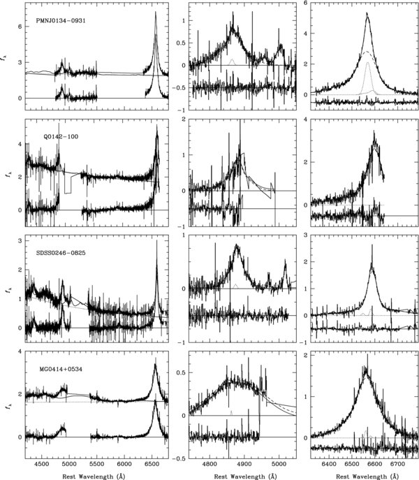
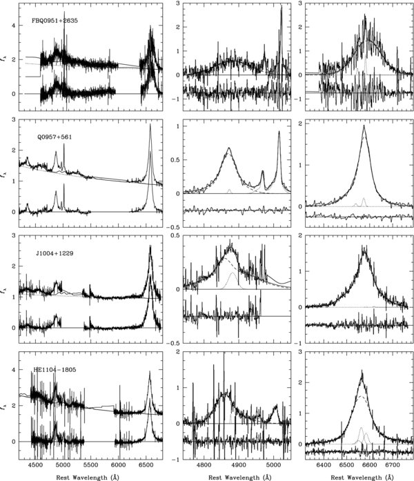
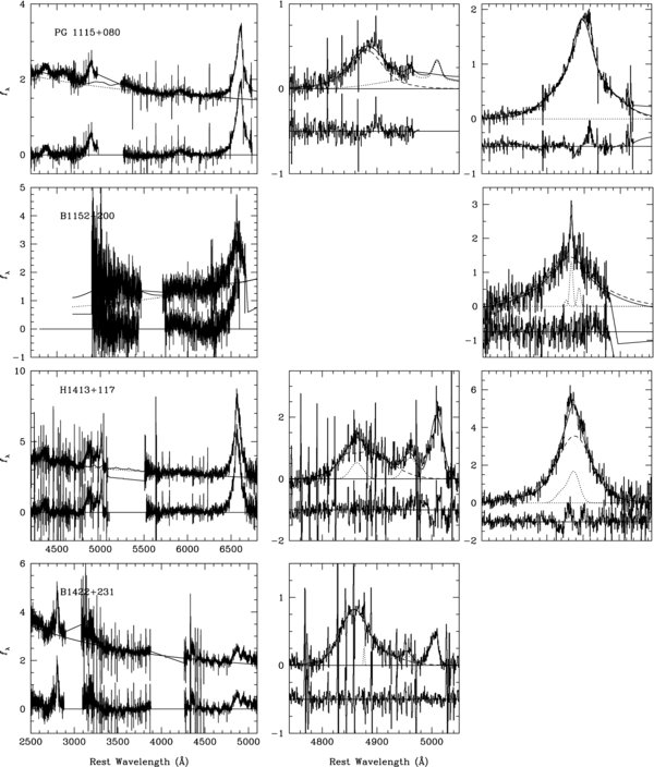
In practice, we fit the power-law continuum, Fe ii emission, and Balmer continuum simultaneously, using emission-line–free windows (see Figure 1). The fits include a normalization and slope for the (single) power-law component, a width, shift, and amplitude for the Fe template, and a density and optical depth for the Balmer continuum. In the UV, we find the best results fixing the Fe ii broadening to that of Hβ, while in the optical we find negligible difference in allowing the broadening to be free. We subtract the continuum model and create a line-only spectrum.
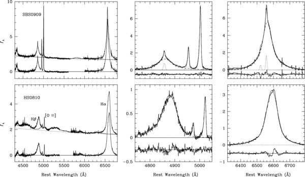
Figure 1. Example fits to the continuum (left), Hβ (middle), and Hα (right) lines from the Triplespec data. We show the data (solid histogram), the total model (thin solid), the broad- (dashed) and narrow-line (dotted) model components, and residuals below (thin solid histogram). Data are plotted with an arbitrary scale in _f_λ. The rest of the sample are plotted in the appendix.
Download figure:
Standard imageHigh-resolution image


We fit the emission line spectra with multi-component Gaussians. These components are used only to create a high-fidelity noise-free match to the emission lines; we do not ascribe physical meaning to them. We first fit the Hβ+[O iii]λλ4959, 5007 region. The narrow [O iii] lines are fit with up to three Gaussians each, with the relative wavelengths tied to laboratory values and the line intensities constrained to have a flux ratio of 1:3 (Table 2; see details in Greene & Ho 2005a; Greene et al. 2009). The width of the narrow Hβ line (fit with a single Gaussian) is tied to that of [O iii] whenever possible (Table 3).5 Finally, broad Hβ is fit with up to four (typically two) broad components. We also find the need to impose a lower limit of 1000 km s−1 on the broad components so that they do not erroneously fit a narrow-line component. We note that in these bright quasars the flux contribution from the narrow lines is typically small. Nevertheless, the treatment of the narrow lines is a source of uncertainty in the FWHM measurements, particularly in the UV. As described below, we therefore perform an additional fit with no narrow component and fold the difference into our total error budget.
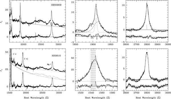
Figure 2. Example fits to the continuum (left), C iv or C iii] (middle), and Mg ii (right) lines from the SDSS data, shown in units of 10−15 erg s−1 cm−2 Å−1. We show the data (solid histogram), the total model (thin solid), the broad- (dashed) and narrow-line (dotted) model components, and residuals below (thin solid histogram). The dashed vertical lines denote a masked region of the spectrum that is heavily absorbed in the original spectrum. Note that in the C iii] profile (top-middle panel) we show only the broad component of the C iii] line itself.
Download figure:
Standard imageHigh-resolution image


Table 3. Line-width Measurements
| Name | z | FWHM[O iii] | FWHMHα | FWHMHβ | FWHMMg ii | FWHMC iii] | FWHMC iv | λ_L_5100 Å | log _M_BH,P06 | log _M_BH,Hα | log _M_BH,Hβ |
|---|---|---|---|---|---|---|---|---|---|---|---|
| (1) | (2) | (3) | (4) | (5) | (6) | (7) | (8) | (9) | (10) | (11) | (12) |
| PMNJ0134 − 0931 | 2.22 | 1410 | 5.1 ± 0.5 | 4.2 ± 1.4 | … | … | … | … | … | … | … |
| Q0142 − 100 | 2.7 | … | 3.8 ± 0.3 | 2.7 ± 0.6 | … | 6.0 ± 0.2 | 6.5 ± 1.3 | 46.42 | 9.4 | 9.4 ± 0.3 | 9.1 ± 0.4 |
| SDSS0246 − 0825 | 1.69 | 540 | 2.5 ± 0.2 | 2.5 ± 0.6 | 2.9 ± 0.1 | 4.5 ± 2.8 | 5.0 ± 0.2 | … | … | … | … |
| MG0414+0534 | 2.6 | … | 5.3 ± 0.3 | 10.8 ± 2.3 | … | … | … | 45.73 | 9.3 | 9.4 ± 0.3 | … |
| HS0810+2554 | 1.51 | 490 | 3.8 ± 0.0 | 4.4 ± 1.1 | 3.6 ± 0.1 | 4.6 ± 0.4 | 3.9 ± 0.1 | … | … | … | … |
| SBS0909+523 | 1.38 | 410 | 3.1 ± 0.6 | 4.1 ± 1.6 | 3.5 ± 0.5 | 4.1 ± 1.1 | … | 45.96 | 9.6 | 9.0 ± 0.3 | 9.2 ± 0.5 |
| FBQ0951+2635 | 1.25 | 290 | 6.3 ± 0.4 | 7.6 ± 0.8 | 6.0 ± 0.3 | 7.2 ± 0.8 | … | 45.48 | 8.9 | 9.4 ± 0.3 | 9.5 ± 0.3 |
| Q0957+561 | 1.41 | 570 | 3.0 ± 0.2 | 3.3 ± 0.9 | 3.3 ± 0.2 | 5.2 ± 0.5 | … | 46.25 | 9.3 | 9.1 ± 0.3 | 9.2 ± 0.4 |
| J1004+1229 | 2.7 | … | 3.8 ± 0.1 | 5.9 ± 1.5 | … | … | … | 46.12 | 9.3 | 9.3 ± 0.3 | 9.6 ± 0.4 |
| HE1104 − 1805 | 2.32 | 970 | 4.7 ± 0.2 | 3.8 ± 0.9 | … | … | … | 45.59 | 9.4 | 9.2 ± 0.3 | 8.9 ± 0.4 |
| PG1115+080 | 1.7 | … | 4.0 ± 0.1 | 4.4 ± 0.2 | 4.0 ± 0.2 | 5.7 ± 3.1 | 6.7 ± 1.0 | 45.15 | 9.0 | 8.8 ± 0.2 | 8.8 ± 0.3 |
| B1152+200 | 1.0 | … | 7.1 ± 2.6 | … | … | … | 3.3 ± 0.6 | … | … | … | … |
| H1413+117 | 2.55 | 1650 | 5.3 ± 0.8 | 6.7 ± 1.9 | … | 8.0 ± 3.2 | 3.3 ± 0.6 | 45.67 | 8.4 | 9.3 ± 0.3 | 9.5 ± 0.3 |
| B1422+231 | 3.63 | 2720 | … | 6.1 ± 2.2 | … | … | … | 46.65 | 9.7 | … | 9.9 ± 0.4 |
| FBQ1633+3134 | 1.52 | 1720 | 4.1 ± 0.7 | 4.6 ± 0.9 | 4.1 ± 0.5 | 6.4 ± 0.6 | 3.8 ± 0.7 | 45.81 | 9.2 | 9.2 ± 0.3 | 9.2 ± 0.6 |
| Q2237+030 | 1.70 | 1070 | 4.8 ± 0.6 | 3.8 ± 1.4 | … | … | … | … | … | … | … |
Notes. Column 1: name; Column 2: redshift. Cases with three significant digits were measured from [O iii], while cases with two come from the Castles website (http://www.cfa.harvard.edu/castles/). See P06 for references. Column 3: FWHM of [O iii] λ5007 Å line (km s−1), with the instrumental resolution of σ* ≈ 36 km s−1 subtracted in quadrature. Column 4: FWHMHα (103 km s−1) measured from the Triplespec data. Column 5: FWHMHβ (103 km s−1) measured from the Triplespec data. Asterisks denote objects with incomplete spectral coverage of the Hβ line. Column 6: FWHMMgII (103 km s−1) measured from the SDSS spectrum. Column 7: FWHMCIII] (103 km s−1) measured from the SDSS spectrum. Column 8: FWHMCIV (103 km s−1) measured from the SDSS spectrum. Column 9: monochromatic luminosity (erg s−1) at λ = 5100 Å as measured from photometry (P06). Column 10: Log (_M_BH/_M_☉) from P06; typically based on the C iv line. We do not quote errors in the BH masses, since systematic uncertainties dominate. We typically quote a factor of 4 error as derived by Vestergaard & Peterson 2006. Column 11: Log (_M_BH/_M_☉) calculated using Equation (1) and the FWHMHα from Column 4 combined with the luminosity from Column 9. Note that the errors in the Hα masses shown here include only measurement uncertainties. Column 12: Log (_M_BH/_M_☉) based on Hβ. In this case Equation (2) and FWHMHβ from Column 5 are combined with the luminosity from Column 9.
Download table as: ASCIITypeset image

Our approach is similar in the case of the Hα+[N ii] complex (see also Ho et al. 1997; Greene & Ho 2004). Here we fix the narrow Hα and [N ii] to the [O iii] line width, fix the relative wavelengths to laboratory values, and fix the relative strengths of the [N ii]λλ6548, 6584 Å to 1:3. In cases where there is no [O iii] line, we fix the narrow-line width to 500 km s−1. Generally in these cases the narrow components are too weak to be fit independently. Uncertainties in this procedure are estimated using an alternate fit with no narrow-line components. We fit the broad Hα with as many as four Gaussians, but do not tie them to the Hβ profile in any way. All of the Triplespec spectra and fits are shown in Figure 1 and the Appendix.
Our fits to the UV lines proceed in a similar fashion, with each broad line modeled as the sum of up to four Gaussians. We still choose to tie the narrow-line components to the width of [O iii] as above, although we note that the proper treatment of the narrow component of C iv remains a matter of debate in the literature (Baskin & Laor 2005; Vestergaard & Peterson 2006; Kelly & Bechtold 2007; Shen et al. 2008b). Again, in cases without available [O iii] fits, we have simply chosen a representative width of 500 km s−1, and again we perform a second, narrow-line-free, fit. Finally, we include a linear continuum component to remove residual continuum errors (Figure 2). We note that the quality of the Mg ii fit does depend on the Fe ii subtraction, and our model for the Fe ii continuum is poorly constrained directly beneath the Mg ii line. However, numerous authors have now shown that the uncertainty in FWHM incurred by differing Fe ii models is small (<0.02 dex; Salviander et al. 2007; Fine et al. 2008).
In addition to the standard Mg ii and C iv lines, we have attempted to model the C iii]λ1909 transition, since it seems worth investigating every possible transition in the UV (and at least in one object, reverberation mapping with this line yielded a mass that is consistent with other transitions; Onken & Peterson 2002). There are good reasons to avoid C iii], including blending with S iii]λ1892, Al iiiλ1857, and Fe iii multiplets (e.g., Dietrich et al. 2002). To minimize these degeneracies, each of the three lines (C iii], S iii], and Al iii) is modeled as a single Gaussian with the same width. The relative centroids are fixed to laboratory values and the strengths are left free. We include a narrow component only for C iii], and it is fixed to the [O iii] width as above. Although we also attempted to include the Fe iii multiplets (Vestergaard & Wilkes 2001) in the fit, keeping the width constrained to that of the Fe ii multiplets, the results were not well constrained. It can be seen in Table 3 that, unexpectedly, in three out of six cases FWHMC iii] is larger than FWHMC iv. However, these are systems with narrow or broad absorption-line systems, which make the C iv fits particularly uncertain.
After fitting, our velocity measure of choice is a non-parametric full-width at half-maximum (FWHM) derived from our multi-Gaussian fits. We are aware that many authors advocate the use of the line dispersion rather than the FWHM (e.g., Peterson et al. 2004; Onken et al. 2004; Denney et al. 2009a). We do not believe there to be a strong argument in favor of one or the other line-width measurement at the current time (although see Collin et al. 2006), but we do know that our technique is robust in the presence of noisy spectra, even when fitting thousands of spectra. We direct the interested reader to the appendix of Greene & Ho (2007a) for a detailed explication of our reasoning, but see also Denney et al. (2009a).
3.2. Linewidth Comparisons
In this subsection, we present figures comparing various estimates of line width derived from different elemental transitions (Figures 3–6). It is clear from these figures that measurement uncertainties alone lead to a significant amount of scatter and that the total dynamic range in line width for any transition is only a factor of ≲3 (e.g., Fine et al. 2008; Shen et al. 2008b).
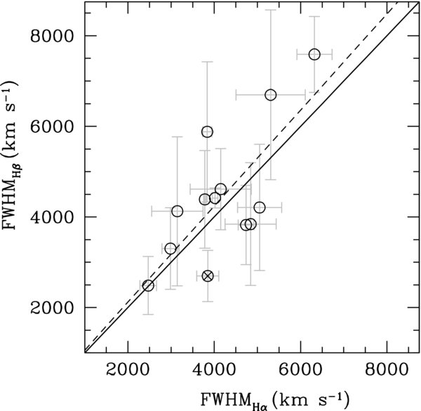
Figure 3. Comparison between the line widths derived from Hα and Hβ in the Triplespec data. Hβ lines with incomplete spectral coverage are noted with a cross. The one-to-one line (solid) is shown for reference only. As expected (e.g., Greene & Ho 2005b) Hβ is generally broader than Hα. Excluding the compromised Hβ fits, we find 〈FWHMHα/FWHMHβ〉 = 0.9 ± 0.2 (dashed line), which is consistent with the 7% difference in line width found by Greene & Ho (2005b), albeit with considerable scatter. We note that MG0414+0534 has a very large and very unreliable Hβ line that is off the scale of this plot.
Download figure:
Standard imageHigh-resolution image


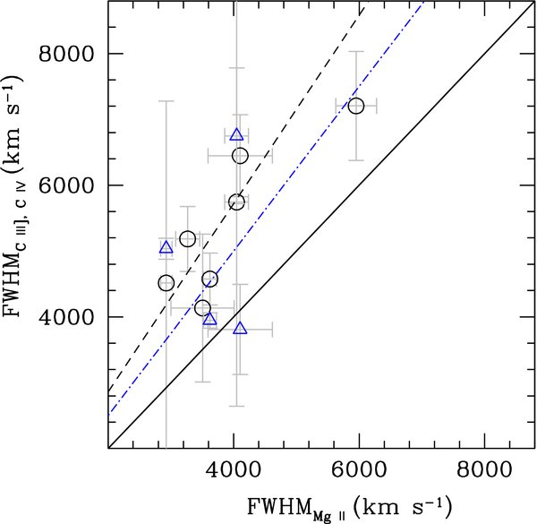
Figure 4. Comparison between the line widths derived from Mg ii and C iii] (black open circles) or C iv (blue open triangles) from the SDSS data. The one-to-one line (solid) is shown for reference only. We find 〈FWHMMg ii/FWHMC iii]〉 = 0.7 ± 0.1 (black dashed line) and 〈FWHMMg ii/FWHMC iv〉 = 0.8 ± 0.2 (blue dot-dashed line).
Download figure:
Standard imageHigh-resolution image


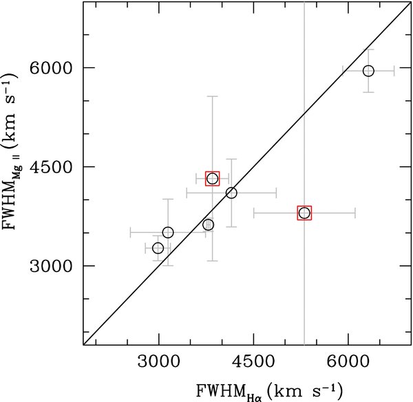
Figure 5. Comparison between the line widths derived from Hα and Mg iii or a scaled C iii] using a ratio of 0.7 (Figure 4) when necessary (red open squares). As above, we show the one-to-one relation as a solid line. Within the scatter, the two measures agree, with 〈FWHMHα/FWHMMg ii〉 = 1.0 ± 0.2.
Download figure:
Standard imageHigh-resolution image


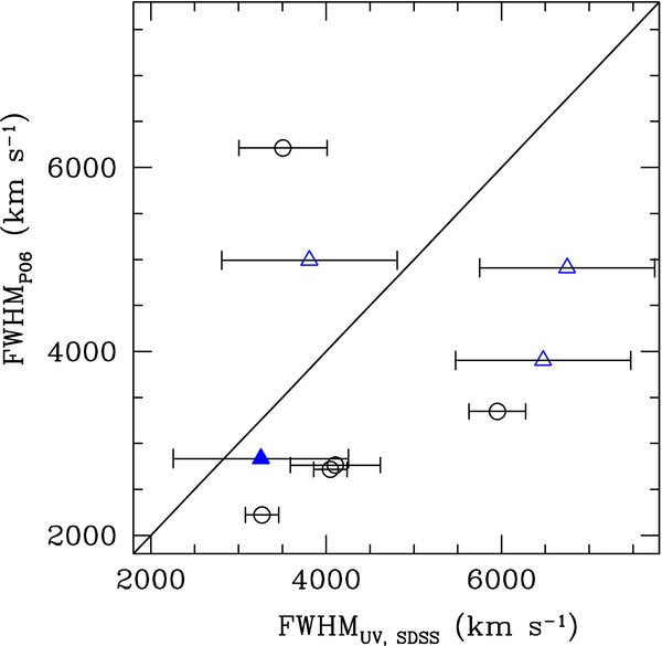
Figure 6. Comparison between our measured UV line widths from Mg ii (black open circles) or C iv (blue open triangles) and those published in P06. Again, the scatter is quite large 〈FWHMMg ii/FWHMP06〉 = 1.5 ± 0.5, and again the unity relation is shown as a solid line. Our tendency to derive broader line widths than P06 derives from our continuum subtraction and treatment of the narrow lines. H1413+117 is highlighted as a filled square because the broad absorption feature in the C iv line makes fitting difficult.
Download figure:
Standard imageHigh-resolution image


For each comparison figure, we have calculated the mean and standard deviation in the ratio of the two lines (not the error in the mean). These numbers are quoted in the figure captions. We have also calculated non-parametric correlation coefficients for each line pair. However, presumably because the samples are so small, none of the correlations are formally significant.
We cannot come to any strong conclusions based on these comparisons, due to both the small sample size and the large measurement errors. We confirm that Hβ is typically broader than Hα (Figure 3; e.g., Greene & Ho 2005b, and references therein). It has long been known that high-ionization lines such as C iv are typically broadened and blueshifted compared to, e.g., Mg ii and the Balmer lines (e.g., Gaskell 1982; Osterbrock & Shuder 1982; Baldwin et al. 1996). While our observations are consistent with that trend (Figure 4), we cannot say much more than that. Over this limited range, we do not see strong evidence of a correlation between the widths of the Balmer lines and C iv, but to a large degree the scatter is driven by the difficulty in measuring a reliable width for the broad-absorption system in H1413+117. Furthermore, the (few) C iii] measurements we have seem to be correlated with the Mg ii line widths (Figure 4). We believe C iii] merits investigation with a much larger sample. Finally, we tend to derive somewhat broader line widths than P06 from the UV lines, presumably because we have subtracted the Fe ii emission, which P06 could not do (Figure 6). In a couple of cases the difference in narrow-line treatment also plays a role. We plan to revisit the UV-based mass estimates for the entire sample using modern spectroscopy (e.g., from SDSS) in future work.
3.3. Mass Estimates
The primary goal of our study is to remove any potential systematic bias in the C iv-based masses presented in P06 by calculating Balmer-based virial masses. In calculating Hα-based BH masses, we start with the radius–luminosity relation of Bentz et al. (2009a). Since this relation was calibrated using Hβ, we then convert FWHMHβ to FWHMHα using the relation derived in Greene & Ho (2005b), which both increase the scaling with FWHMHα to the 2.06 power and slightly changes the prefactor. Finally, for consistency with P06, we assume a scaling factor that is 1.8 times higher than the assumption of isotropic random motions, (e.g., Onken et al. 2004; Greene & Ho 2006) yielding
The masses calculated using this formalism are displayed in Table 3 and Figure 7(a). Note that in the case of B1422+231, Hα is outside our observing window. In this case, we use the Hβ line and the following (very similar) formalism:
The Hβ masses are presented in Figure 7(b).
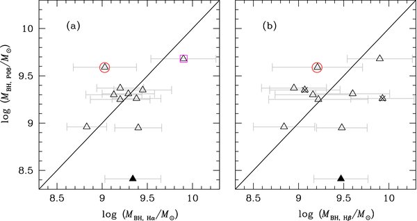
Figure 7. (a) We compare BH mass estimates based on the Hα transition with those from P06. The P06 masses are based on C iv with one exception (red open circle; Mg ii) while our masses are based on Hα with one exception (magenta open square; Hβ). The unity relation (solid line) is shown to guide the eye. While the two mass estimates are not strongly correlated, we do not find any evidence for a systematic offset between the two (the median _M_Hα/_M_P06 = 1.0 ± 0.4). H1413+117, due to its broad-absorption system, is highlighted as a filled symbol. (b) Same as (a), except using Hβ as the virial indicator. In this case, objects with only partial observations of the Hβ line are highlighted with crosses. As above the P06 mass that is based on Mg ii is identified with a red circle. We find a median _M_Hβ/_M_P06 = 1.0 ± 0.5. The filled triangle is H1413+117.
Download figure:
Standard imageHigh-resolution image


The luminosities used here are derived from the Hubble Space Telescope (HST) photometry of the CASTLES sample, as described in detail in P06. Briefly, the quasar and host galaxy images are optimized along with the lens model using LENSFIT (a variant of GALFIT; Peng et al. 2002). The quasars are modeled as point sources, the galaxies as Sérsic (1968) functions, and the lensing masses as singular isothermal ellipsoids. The demagnified and deblended V, I, H quasar magnitudes are modeled as a power law, with the slopes presented in Table 2, and the luminosities come from this fit. We note that our spectroscopically derived slopes agree nicely with those from broadband photometry. We find 〈αopt/αP06〉 = 1 ± 0.5, where _f_λ ∝ λα. The HST _H_-band images correspond closely to rest-frame _V_-band at z ≈ 2, so the luminosities are very insensitive to uncertainties in the power-law slope.
We find a mean ratio of 〈log(_M_Hα/_M_P06)〉 = −0.02 ± 0.5 between the two mass estimates. Although the scatter is large, we find no evidence for a systematic offset in the C iv-based masses. Therefore, to the extent that virial mass estimates have merit in this mass, luminosity, and redshift regime (as yet untested directly), our new spectroscopic observations confirm the results presented in P06.
3.4. Uncertainties
Uncertainties in line widths are difficult to estimate. In our case, the signal-to-noise (S/N) ratios of the spectra are not very high (see Table 1), which contributes substantially to the error budget. We use Monte Carlo simulations to estimate the magnitude of the uncertainties due to finite S/N. For each observed line, we generate 1000 mock spectra with the same shape as our best-fit model and the same noise as our observed spectrum. In order to model residual uncertainties in continuum subtraction, we include a broadened Fe ii spectrum with an amplitude that scatters around 10% of the peak flux. Using the same procedures as in the real data, we then measure the best-fit parameters for each of these simulations. The uncertainty is determined from the distribution of simulated line dispersion to be half of the width encompassing 68% of the simulated galaxy measurements, and ranges from ∼10%to40% of the measured value. Now, in addition to noise, the treatment of narrow emission lines can be a significant cause of systematic uncertainty. Thus, we perform a second fit with the narrow component of each line turned off, and the difference between the two represents a second estimate of the uncertainty. We adopt the larger of these as our final error in line width.
At the same time, quasar variability adds additional uncertainty, since the rest-frame optical and UV spectra analyzed here were not obtained contemporaneously. Wilhite et al. (2007) and Denney et al. (2009a) both find that variability in line width tends to be small (∼30%) and thus only contributes ∼0.1 dex scatter to BH mass estimates. Another feature of quasar spectra that complicates emission-line-width measurements is the presence of blueshifted absorption features with velocity widths of tens (narrow) to tens of thousands (broad) of km s−1. Both H1413+117 and (to a lesser extent) PG1115+080 display broad absorption features, while Q0957+561 and HS0810+2554 have significant narrow absorption. In these cases, we simply mask the regions from the fit, but note that particularly in the case of H1413+117, our ability to measure a reliable C iv width is seriously compromised, since even the line center is not well defined.
In addition to the line widths presented here, the BH masses depend on the luminosity of the quasar. We briefly review the arguments that the lens modeling does not add significant uncertainties to our results and direct the interested reader to Appendix B of P06 for more details. The primary source of uncertainty in the models is that gravitational time delay and lensing substructures can lead to anomalous quasar magnification ratios, which translate into an uncertainty in the quasar luminosity. However, this error should be no larger than 0.1–0.2 mag, and thus does not contribute significantly to the BH mass uncertainty. Actual measurement uncertainties from model fitting are tiny for the quasar.
In Table 3, we present the formal uncertainties in BH mass arising from errors in the FWHM measurements and the formal uncertainty in the slope of the radius–luminosity relation. We wish to emphasize that the true errors in BH mass are probably dominated by systematic uncertainties arising from our ignorance of the structure and kinematics of the BLR that translate into errors in inferring both its true extent and velocity field based on the observations (Krolik 2001; Collin et al. 2006; Greene & Ho 2006). At present, we really have no concrete confirmation that (1) the same radius–luminosity relation applies to quasars at these luminosities (although see Kaspi et al. 2007) nor that (2) it is meaningful to assume that the BLR gas is in virial equilibrium and not, for instance, dominated by a massive outflow (e.g., Baldwin et al. 1996; Richards et al. 2002a; Leighly & Moore 2004; Fine et al. 2008).
To summarize, we have obtained Hα-based BH masses for a large fraction of the lensed quasars with measured host galaxy luminosities from P06. While the scatter between Hα-based and C iv- or Mg ii-based BH masses is quite large (∼0.5 dex), we do not see evidence for a systematic bias in mass. Thus, we do not alter the result of P06 that _M_BH–_L_bulge relations appear to evolve with cosmic time.
It is instructive to now compare the properties of the lensed sample with the general quasar population at 1 ≲ z ≲ 4. A large number of studies have looked at the distributions of BH mass and Eddington ratio of luminous quasars (e.g., McLure & Dunlop 2004; Kollmeier et al. 2006; Netzer et al. 2007; Fine et al. 2008; Shen et al. 2008b; Gavignaud et al. 2008) including some work on narrow-line quasars (Greene et al. 2009; Liu et al. 2009) as well as mass functions for quasars (e.g., Greene & Ho 2007b; Vestergaard et al. 2008; Kelly et al. 2009). In most cases, the BH masses are based on C iv and Mg ii from observed optical spectra. Generally, all works find the same surprisingly narrow range in measured line width, and correspondingly narrow distributions in _M_BH and _L_bol/_L_Edd at all redshifts (although as Gavignaud et al. point out, the derived distribution is quite sensitive to the assumed slope in the radius–luminosity relation).
For our purpose, it is easiest to compare with the results of Netzer et al., as their study is also based on Hβ observations. For convenience, we adopt their assumption that _L_5100 Å is ∼one seventh of the bolometric luminosity and we take the Eddington luminosity to be 1.26 × 1038 (_M_BH/_M_☉) erg s−1. Despite completely different selection criteria, the distributions in luminosity, and correspondingly inferred BH mass and Eddington ratio, are quite similar across the two samples (Figure 8). For the Triplespec sample, the median 〈_M_BH〉 ≈ 2 × 10⁹ _M_☉ and the median _L_5100 Å≈6 × 1045 erg s−1 yield a typical Eddington fraction of ∼30%. If we take the entire P06 sample, using Hα-based masses when available, we find a median mass of ∼109 _M_☉, a median _L_5100 Å of 2 × 1045 erg s−1, and a median Eddington ratio of 10%.
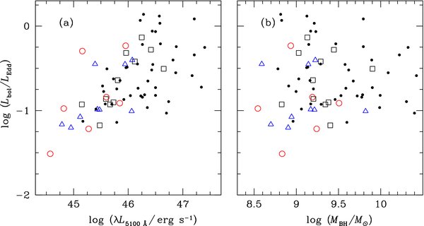
Figure 8. (a) We reproduce Figure 2 from Netzer et al. (2007, black dots_; based on_ _H_β) and include the targets from this study (large black open squares), as well as the entire P06 sample, differentiating between Mg ii-based (small red circles) and C iv-based (small blue triangles) masses. Here we plot monochromatic 5100 Å luminosity vs. the Eddington ratio. We follow Netzer et al. and assume that the bolometric luminosity is 7 times _L_5100 Å. Both our mass estimates and those from Netzer et al. are based on Balmer emission lines (Hβ in their case). (b) _M_BH vs. _L_bol/_L_Edd; symbols as in (a). We see that the distributions in each diagram are similar between the two samples, although the lensed systems extend to objects that are factors of 2–3 times fainter.
Download figure:
Standard imageHigh-resolution image


Unlike other studies, Netzer et al. actually argue that their sample displays a broad distribution in the Eddington ratio when compared to theoretical expectations that luminous quasars should be most readily observed at or near their Eddington luminosities (e.g., Marconi et al. 2004; Merloni 2004; Hopkins et al. 2006). We find the observed distributions unexpected for a somewhat different reason, namely the uniformly high BH masses. Assuming that the Eddington limit strictly applies and given the lower flux limit of the lensed sample, we could detect BHs with masses as low as ∼108 _M_☉. Furthermore, our intuition from the local BH mass function (e.g., Yu & Tremaine 2002; Marconi et al. 2004) suggests that 108 _M_☉ BHs ought to be far more numerous than 109 _M_☉ systems due to the exponential decline in the space density of the most luminous galaxies. Given that supercritical accretion may be observed locally (e.g., Pounds et al. 1995; Mineshige et al. 2000; Desroches et al. 2009), we find the preponderance of ∼109 _M_☉ BHs radiating at ∼10% of their Eddington luminosity to be noteworthy.
We can be slightly more quantitative. Following, e.g., Somerville (2009), we can transform the observed z ∼ 2 galaxy mass function (e.g., Fontana et al. 2006) into the expected BH mass function. For reference, at the median luminosity of the Triplespec sample, the Eddington limit sets a bound of ∼4 × 10⁸ _M_☉ on observable BHs. If the relation between _M_BH and galaxy mass were identical to what it is today (e.g., Gültekin et al. 2009), then the BHs with mass ≈4 × 10⁸ _M_☉ ought to be ∼50 times more common than the median observed mass of _M_BH ≈2 × 10⁹ _M_☉. Note that we are conservatively adopting the median rather than the minimum observed luminosity and assuming that the Eddington luminosity applies strictly. Taking the observed masses at the face value for the moment, and assuming that the selection of lensed quasars is simply a random selection of optically luminous quasars at 1 < z < 4, we infer that either BHs radiating at 30% of Eddington are ∼50 times more numerous than Eddington-limited objects or that the zero point in the _M_BH–_L_bulge relation has evolved by a factor of ∼3 to the present day. This latter, of course, is the suggestion made by P06.
Obviously, such constraints are not particularly stringent at the moment. For one thing, the selection of lensed quasars is complicated to model, involving radio selection in some cases (which will tend to bias samples toward more massive systems; e.g., Heckman 1983; Mandelbaum et al. 2009). Furthermore, as pointed out by Somerville, joint constraints from galaxy and quasar luminosity functions on their own cannot distinguish between zero-point evolution or increased scatter in BH–bulge relations at high redshift. Finally, we do not know that the quasar duty cycle is independent of mass. Nevertheless, we cannot help but wonder whether the narrow range in observed line width, and the unexpectedly high average BH mass, do not instead indicate a problem in virial mass estimators at high luminosity that may be resolved with better understanding of the physics of broad-line quasars.
Ultimately, the question is whether or not the broad emission lines in luminous quasars are dominated by virial motions. Of course, there is evidence for a non-virialized component in the C iv line (e.g., Baldwin et al. 1996; Richards et al. 2002a). On the other hand, there is clear evidence for virialized motion in the BLRs of at least a few nearby lower luminosity active galaxies (e.g., Peterson & Wandel 1999; Onken & Peterson 2002; Peterson et al. 2004). Also, the local virial masses seem to correlate with both σ* (e.g., Shen et al. 2008a) and _L_bulge (e.g., Kim et al. 2008b; Bentz et al. 2009b). Unfortunately, similar analysis is not yet available in the luminosity range of interest to us. At present, all we can say is that the C iv-based masses alone are not causing a net bias in the virial masses relative to the Balmer lines. True evolution in BH–bulge scaling relations is by no means certain; far more pernicious sources of uncertainty remain, including potential biases in sample selection. At the minimum, to mitigate these concerns, quasar samples with identical selection at multiple redshifts are needed.
In closing, we note that BH–bulge relations are not the only ones purported to display unexpected evolution since a redshift z ≈ 2. Recent work has shown that, at a fixed mass, elliptical galaxies were a factor of 2–5 smaller at redshifts of one and two, respectively, than they are today (e.g., Trujillo et al. 2006; van Dokkum et al. 2008; Franx et al. 2008; van der Wel et al. 2008; Damjanov et al. 2009). At first it seems counterintuitive that the most massive elliptical galaxies, which seem to have formed the bulk of their stars rapidly at an earlier epoch (e.g., Thomas et al. 2005), should grow less dense with time. However, a large number of minor mergers can very efficiently build the outskirts of elliptical galaxies (e.g., Boylan-Kolchin & Ma 2007; Bezanson et al. 2009; Naab et al. 2009). Interestingly, these gas-free minor mergers would need to grow the total galaxy mass by factors of 2–3 in order to match local observations (e.g., Bezanson et al. 2009). This is possible under a scenario where the BH-to-TOTAL stellar mass relation is steeper than linearity in low-mass galaxies, which is observed in nearby galaxies (Gültekin et al. 2009; Greene et al. 2008). In gas-free merging, there is no corresponding BH growth via accretion, which could facilitate a boost in the BH–bulge ratio at late times (see also Hopkins et al. 2009). As argued by Peng (2007), numerous minor mergers will tend to drive the ratio of BH to galaxy mass toward a value of unity slope (e.g., his Figure 2(b) and 4(a)). Alternatively, as suggested by both Croton (2006) and Jahnke et al. (2009), it may be that disk components are common in the high-redshift galaxies but are subsequently subsumed into the main elliptical galaxy body. We mention this apparent coincidence in passing because it is intriguing, although we note that a variety of outstanding uncertainties are yet to be explored as far as the structural evolution of elliptical galaxies is concerned.
We revisit the BH mass estimates for a sample of lensed quasars with high-fidelity host-galaxy luminosities from Peng et al. (2006b). While the Balmer-based masses presented here are arguably more robust than the UV-based estimates, we find no evidence for a systematic difference in BH masses based on the two methods. If we can take the Balmer-based virial masses at the face value, then we confirm the result of Peng et al. (2006b) that BHs appear to be overly massive relative to their hosts at high redshift. Intriguingly, the minor mergers that are invoked to puff up compact elliptical galaxies at late times would be very effective at boosting the galaxy to BH mass ratio as well. However, as pointed out many times, the persistently narrow range in observed line width for luminous quasars at high redshift provides substantial cause for concern in the veracity of the virial masses. Furthermore, it is not clear that we have yet assembled consistent comparison quasar samples across cosmic time with which to compare the BH–bulge scaling relations. Our work is a necessary, but not sufficient, step in determining the true evolution of BH–bulge relations with cosmic time.
The referee provided a very careful and insightful reading that substantively improved the manuscript. Both J.E.G. and C.Y.P. are grateful for many stimulating conversations with L.C.Ho, and we thank A. J. Barth and C. A. Onken for very useful comments. We thank M. Skrutskie for taking commissioning data for this project and for invaluable help with the reduction software. We thank H. Netzer for kindly providing his data table for Figure 8. Support for J.E.G. was partially provided by NASA through Hubble Fellowship grant HF-01196 awarded by the Space Telescope Science Institute, which is operated by the Association of Universities for Research in Astronomy, Inc., for NASA, under contract NAS 5-26555.
In Figure A1(a–d), we present the rest of the Triplespec spectra for completeness. Note that the Triplespec spectra for SBS0909 and HS0810 are shown in Figure 1.
Download figure:
Standard imageHigh-resolution image


Download figure:
Standard imageHigh-resolution image


Download figure:
Standard imageHigh-resolution image


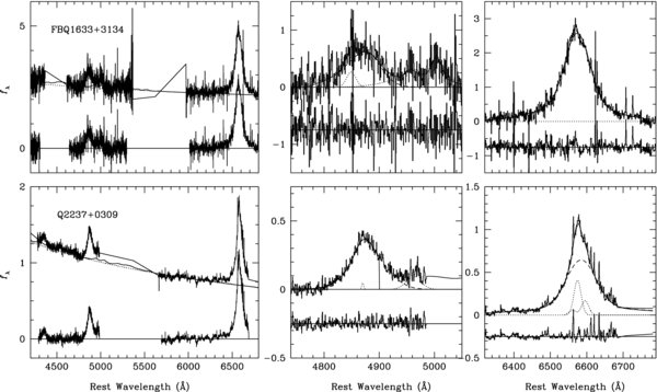
Figure A1. Fits to the continuum (left), Hβ (middle), and Hα (right) lines from the Triplespec data that do not appear in Figure 1. We show the data (solid histogram), the total model (thin solid), the broad- (dashed) and narrow-line (dotted) model components, and residuals below (thin solid histogram). Data are plotted with an arbitrary scale in _f_λ. Spectral regions that are masked in the fit do not appear in the residuals (e.g., the red wing of Hβ for Q0142-100). Also note that in a couple of cases the [O iii] fit is based exclusively on the λ4959 line; no redshifts are derived for these targets.
Download figure:

