Land-based climate change mitigation potentials within the agenda for sustainable development (original) (raw)
The Sustainable Development Goals (SDGs) set an agenda for the sustainable management of social, physical, and ecological elements of the Earth system and attempt to guide and monitor progress along 17 goals and 169 specific targets (Griggs et al 2013). Among SDGs, climate change mitigation received much attention in the past and with the Paris Agreement momentum was increased. To stabilize the climate possibly below 1.5 °C above pre-industrial levels, large contribution across all economic sectors including agriculture and forestry is required (IPCC 2018, Rogelj et al, 2018, Roe et al, 2019). Integrated Assessment Models (IAM) that are used to develop climate stabilization pathways have consistent perception on the net emission profile and energy portfolio required to achieve climate stabilization cost-efficiently (IPCC 2018, Rogelj et al 2018). This has direct implications for the required land-based mitigation efforts (agriculture, forestry and other land use sector—AFOLU) through (i) supply of biomass for bioenergy and (ii) reduction of land use related greenhouse gases (GHGs).
IAMs anticipate an up to fivefold increase in total primary biomass demand for energy by 2050 in the Shared Socio-economic Pathway (SSP)2 to stay on track with the 1.5 °C target (Rogelj et al 2018). Such large scale deployment of bioenergy may trigger environmental and social trade-offs such as increased deforestation and emissions, nitrogen losses, increased irrigation water demand, and food prices without accompanying policies (Calvin et al 2014, Bonsch et al 2016, Humpenöder et al 2018, Hasegawa et al 2020). Hence, biomass based bioenergy production should be deployed sensibly in order to not violate sustainability thresholds (Creutzig et al 2015). In addition, the land use sector, including agriculture and forestry, is expected to deliver mitigation efforts of around 8 GtCO2eq yr−1 by 2050 according to IAMs (Rogelj et al 2018) while other studies estimate even higher land-based mitigation potentials (Griscom et al, 2017, IPCC 2019, Roe et al 2019). However, stringent agricultural GHG mitigation and the need to enhance the land carbon sink i.e. through afforestation, may further increase the cost of agricultural production and competition for land and deteriorate other SDGs such as food security (S Frank et al 2017, Hasegawa et al, 2018, Fujimori et al 2019, IPCC 2019, Peña-Lévano et al 2019).
Aside the importance of the land use sector for successful climate change mitigation (SDG13) (Grassi et al 2017, Harper et al, 2018, Roe et al 2019), developments in the sector are also closely tied to the achievement of many SDGs (IPCC 2019, IUFRO 2019), in particular SDG2 Zero Hunger, SDG6 Clean Water and Sanitation, SDG12 Responsible Consumption and Production, and SDG15 Life on Land (Obersteiner et al, 2016). Operationalizing the contribution from land use to climate stabilization while ensuring coordination across SDGs is challenging and complex (Obersteiner et al 2016, Grassi et al 2018, Brown et al 2019). Recent studies raised awareness to sustainability issues related to ambitious climate stabilization pathways (Bonsch et al 2016, Heck et al 2018, Humpenöder et al 2018, Obersteiner et al, 2018). Still, current climate stabilization transition pathways focused so far mainly on the overall feasibility of reaching the 1.5 °C target and assessed SDG trade-offs/synergies from an economy-wide perspective (Bertram et al 2018, Grubler et al, 2018, Rogelj et al 2018, van Vuuren et al, 2018).
Here we apply the economic land use model GLOBIOM (Havlík et al, 2014) together with the forest model (G Kindermann et al, 2008a, Gusti 2010). The use of partial equilibrium models with in-depth sectorial and spatially explicit coverage allows to represent biophysical and (socio-) economic aspects across scales and across the land-uses in a consistent bottom–up modelling framework. First, we quantify the economic potentials of agriculture and forestry to contribute to climate change mitigation. We then consider how this potential is affected by pursuing key selected land use related SDG targets by 2030. We explicitly consider limiting undernourishment to 1% (SDG2), reducing livestock calorie intake in overconsuming countries through preference change to 430 kcal capita−1 day−1 (SDG12), halving food waste (SDG12), increasing the share of protected areas to 17% and avoiding conversion of biodiversity hot-spots (SDG15), and respecting environmental water flow requirements for fresh water ecosystems protection (SDG6). These SDGs were selected to achieve broad coverage of land use related SDGs and consider key trade-offs/synergies as identified in the literature (Springmann et al 2016, Hasegawa et al 2018, IPCC 2018,2019, Pastor et al 2019, Leclère et al 2020) in our assessment. First, we assess direct impacts of globally achieving these selected SDGs on the capacity of the land use sector to contribute to mitigation efforts via biomass provision and AFOLU GHG mitigation. We quantify impacts on biomass potentials for bioenergy (sourced from energy plantations, and forests including primary and secondary forest residues), on AFOLU mitigation potentials (CO2, CH4, and N2O) and assess interdependencies among these two key land-based mitigation portfolios. The quantified scenario matrix (table 1, and method section) provides a rich dataset/model emulation that can be used by IAMs and in other models, which used similar matrixes in the past however without consideration of the SDG implications (Emmerling et al 2016, Fricko et al, 2016, Keramidas et al 2017), to develop SDG compliant climate stabilization pathways for land use.
Table 1. Quantified scenario matrix to assess interactions between SDGs and land-based mitigation potentials.
| Scenario name | Mitigation strategy a | Sustainable Development Goals | |||||
|---|---|---|---|---|---|---|---|
| SDGs | Mitigation | GHG mitigation (SDG13) | Bioenergy deployment (SDG13) | Food security (SDG2) | Diets and food waste (SDG12) | Irrigation water (SDG6) | Bio-diversity (SDG15) |
| noSDGs | Baseline | ✗ | ✗ | ✗ | ✗ | ✗ | ✗ |
| noSDGs | GHG mitigation | ✓ | ✗ | ✗ | ✗ | ✗ | ✗ |
| noSDGs | Bioenergy | ✗ | ✓ | ✗ | ✗ | ✗ | ✗ |
| noSDGs | Combined | ✓ | ✓ | ✗ | ✗ | ✗ | ✗ |
| FOOD | Combined | ✓ | ✓ | ✓ | ✗ | ✗ | ✗ |
| DIET | Combined | ✓ | ✓ | ✗ | ✓ | ✗ | ✗ |
| WATR | Combined | ✓ | ✓ | ✗ | ✗ | ✓ | ✗ |
| BIOD | Combined | ✓ | ✓ | ✗ | ✗ | ✗ | ✓ |
| SDGs | Baseline | ✗ | ✗ | ✓ | ✓ | ✓ | ✓ |
| SDGs | GHG mitigation | ✓ | ✗ | ✓ | ✓ | ✓ | ✓ |
| SDGs | Bioenergy | ✗ | ✓ | ✓ | ✓ | ✓ | ✓ |
| SDGs | Combined | ✓ | ✓ | ✓ | ✓ | ✓ | ✓ |
aWe estimate the AFOLU capacity for climate change mitigation by quantifying different combinations of land-based mitigation strategies and comparing them to the “baseline“ without climate change mitigation efforts: (i) “GHG mitigation“: abatement potentials emulated by implementing different GHG price pathways, and (ii) “bioenergy“: biomass for bioenergy potentials emulated by implementing different biomass price pathways for bioenergy.
2.1. Modelling framework
We apply GLOBIOM (Havlík et al 2014) and G4M (Kindermann et al 2008a, Gusti 2010). GLOBIOM is a partial equilibrium model of the global agricultural and forestry sectors. Commodity markets and international trade are modelled at the level of 37 aggregate economic regions where prices are endogenously determined at the regional level to establish market equilibrium. The spatial resolution of the supply side relies on the concept of Simulation Units, which are aggregates of 5–30 arcmin pixels belonging to the same altitude, slope, and soil class, and also the same country (Skalský et al 2008). For crops, livestock, and forest products, spatially explicit Leontief production functions covering alternative production systems are parameterized using biophysical models like EPIC (Environmental Policy Integrated Model) (Williams 1995), G4M (Global Forest Model) (Kindermann et al 2008b, Gusti 2010), or the RUMINANT model (Herrero et al, 2013). For the present study, the supply side spatial resolution was aggregated to 2 degrees (about 200 × 200 km at the equator). Land and other resources are allocated to the different production and processing activities to maximize a social welfare function which consists of the sum of producer and consumer surplus. Changes in socio-economic and technological conditions, such as economic growth, population changes, and technological progress, lead to adjustments in the product mix and the use of land and other productive resources. By solving the model in a recursive dynamic manner for 10 yr time steps, decade-wise detailed trajectories of variables related to supply, demand, prices, land use, and AFOLU emissions are generated. GLOBIOM covers major GHG emissions from AFOLU use including N2O from the application of synthetic fertilizer and manure to soils, N2O from manure dropped on pastures, CH4 from rice cultivation, N2O and CH4 from manure management, and CH4 from enteric fermentation, and CO2 emissions/removals from above- and belowground biomass changes for other natural vegetation. CO2 emissions/removals from afforestation, deforestation, wood production in managed forests are estimated by geographically explicit (0.5 × 0.5 degree) model G4M (Kindermann et al 2008a, Gusti 2010) that is connected with GLOBIOM. Afforestation and deforestation decisions are calculated by comparing net present values of agriculture and forestry land uses. Afforestation occurs where it is more profitable than the agriculture and the environmental conditions are suitable for forest growth. Deforestation, in contrast, happens where agriculture net present value plus profit from one-time selling of deforested wood exceeds the net present value of forestry. The net present values are estimated considering agriculture land rents and wood prices obtained from GLOBIOM and price of carbon stored in biomass. The land transitions in G4M are harmonized with GLOBIOM agriculture land demand. G4M simulates forest management aimed at sustainable production of wood demanded by GLOBIOM on regional scale.
2.2. Biomass supply for energy use
GLOBIOM explicitly covers biomass feedstocks from energy plantations and existing forests for energy use. Energy plantations are represented through short rotation tree plantations (SRP) of poplar, willow, or eucalyptus with rotation periods of up to 10 yr. Productivities are based on net primary productivity maps (Cramer et al 1999) and the potential for plantation area expansion is determined by land suitability criteria based on aridity, temperature, elevation, population, and land-cover data, as described in Havlík et al (2011).
GLOBIOM has detailed representation of the forest sector and its supply chains (Lauri et al 2017). The model includes five primary wood products (pulplogs, sawlogs, other industrial roundwood, fuelwood, and logging residues) that can be used as input for material or energy production processes. The current version of the model includes eight final products (sawnwood, plywood, fiberboard, chemical pulp, mechanical pulp, other industrial roundwood, fuelwood, and energy wood) and five byproducts (sawdust, woodchips, bark, black liquor, and recycled wood). Biomass for bioenergy can be sourced from pulplogs, fuelwood, logging residues or forest industry by-products. Detailed information on the forest sector representation is provided in Lauri et al (2014) and (2017).
2.3. AFOLU mitigation options
GLOBIOM/G4M represents a comprehensive set of GHG mitigation options for the AFOLU sector. Structural mitigation options for agriculture are considered in GLOBIOM via a comprehensive set of management systems. In the crop sector, four different crop management systems are differentiated using the EPIC model (Williams 1995). In the livestock sector, also various production systems and livestock species are parameterized (Herrero et al 2013). The detailed representation of production systems allows the model to explicitly represent structural changes in the agricultural sector under a climate policy. Farmers can switch to more GHG efficient management practices on site, reallocate production to more productive areas within a region, or through international trade across regions.
In addition, technological options such as anaerobic digesters, animal feed supplements etc are based on the EPA mitigation option database (Beach et al 2015). Emission reduction potentials (% emission savings), costs (annual costs i.e. direct costs and labour costs, change in input costs, and investment costs i.e. for anaerobic digesters), and potential impacts on productivities (% increase/decrease) were taken from the EPA mitigation options database. Relative emission savings and productivity changes were then applied to the different management systems in the GLOBIOM model to calculate absolute changes in GHG emissions and product output. Mitigation options (characterized by GHG reduction, productivity changes, and economic costs) are implemented in the model as additional management activities which can be applied on top of a production system. Mitigation options are adopted if the economic benefit, i.e. through avoided carbon tax payments, potential productivity changes, exceeds the cost of an option. More detailed information on parameterization of the marginal abatement cost curve for agriculture in GLOBIOM is provided in Stefan Frank et al (2018).
G4M considers the following mitigation options for the forestry sector: reduction of deforestation area, increase of afforestation area, change of rotation length of existing managed forests in different locations, change of the ratio of thinning versus final fellings, change of harvest intensity (amount of biomass extracted in thinning and final felling activity), and change of harvest locations. These activities are not adopted independently by the forest owner since the model manages forest land dynamically and activities affect each other. The model is calculating the economic optimal combination of measures and the introduction of a GHG price gives an additional value to the forest through the carbon stored and accumulated in it which tends to decrease deforestation and increase afforestation. This might not happen at the same intensity though since less deforestation increases land scarcity and might therefore decrease afforestation. The existing forest under a GHG price is managed with longer rotations and expanding harvest to less productive forest. Where possible the model increases the area of forests used for wood production, meaning a relatively larger area is managed relatively less intensively which affects the carbon balance. Forest management activities can also have a feedback on emissions from deforestation because they might increase or decrease the average biomass in forests being deforested and influence biomass accumulation in newly planted forests depending on whether these forests are used for production or not. Market feedbacks and effects of these mitigation options e.g. prolonging rotation are explicitly accounted for as the production of wood to satisfy wood demand has higher priority than the carbon accumulation. In fact, much of the mitigation effects are achieved by structural and geographic relocation of harvesting schedules to increase sequestration while at the same time satisfy market demands.
The estimated AFOLU mitigation potentials include N2O from the application of synthetic fertilizer, manure to soils and dropped on pastures, and from manure management, CH4 from rice cultivation, enteric fermentation, and manure management, CO2 emissions from above- and below-ground biomass changes and dead organic matter related to land use changes and forest management as well as soil carbon emissions from deforestation/afforestation. Remaining soil carbon emissions/removals (aside following afforestation/deforestation) as well as mitigation potentials from wetlands are not considered in this study.
2.4. Model emulator—‘lookup-table’
To assess the contribution of the land use sector to climate change mitigation within the agenda for sustainable development, we quantify a matrix of linear carbon and biomass price trajectories in GLOBIOM that cover the range of prices in existing IAM mitigation pathways. This approach allows to quantify supply functions where the supplied biomass quantity available for bioenergy is a function of the biomass price and conditional on a GHG price. Vice versa we quantify the cost-efficient AFOLU mitigation potential in the form of a marginal abatement cost curves (MACC) conditional on the biomass demand where the emission reduction is a function of the GHG price converted through global warming potential of the non-CO2 gases to cover also methane (CH4) and nitrous oxide (N2O) emissions in addition to carbon dioxide (CO2). The biomass supply curves and MACCs are highly interdependent, for instance: a biomass price remunerating forest harvest for bioenergy may encourage additional afforestation. This will increase the carbon sink of the forest while at the same time providing more biomass for bioenergy production. The quantified scenario matrix (also referred to as ‘lookup-table’) represents a GLOBIOM model emulation and provides a comprehensive and detailed response surface for the land use sector that can also be used in other models to explicitly consider dynamics and interlinkages between biomass use and AFOLU emissions but also other important land use related indicators.
2.5. Scenario development
We quantify the lookup-table for the SSP2 scenario (O’Neill et al 2014, Fricko et al 2016) which depicts a ‘Middle of the Road’ scenario with moderate challenges to mitigation and adaptation. Demand for animal protein is relatively high, due to comparatively strong income and population growth. For food demand projections, income elasticities are calibrated to mimic FAO projections of diets (Alexandratos and Bruinsma 2012). Moderate reductions in food waste and losses over time add to the availability of agricultural products. Technological change for crops is based on 18 crop specific yield responses function to GDP per capita growth estimated for different income groups using a fixed effects model. Fertilizer use and costs of agricultural production increase in proportion with yields. Productivity changes through technological change in the livestock sector and transition towards more efficient livestock production systems takes place at a moderately fast pace. Detailed information on the quantification of SSP2 in GLOBIOM is provided in Fricko et al (2016).
We quantify twelve GHG price (0, 10, 20, 50, 100, 200, 400, 600, 1000, 1500, 2000, and 3000 USD tCO2eq−1) and seven bioenergy price (0, 3, 5, 8, 13, 30, and 60 USD GJ−1) combinations for SSP2 which yield in total 84 scenarios. The carbon and biomass prices are implemented linearly from 2020 onwards and reach their full value in 2100. Maximum GHG price and biomass prices were informed by 1.5 °C climate stabilization scenario results from Integrated Assessment Models (IAM) (Rogelj et al 2018).
We quantify the lookup-table for two set-ups (i) default set-up (noSDGs) without consideration of SDGs beyond current policies, and (ii) a SDG set-up (SDG) including four SDG dimensions that are assumed to be achieved by 2030. In the noSDGs set-up no additional elements are included in SSP2 aside the mitigation policy represented through carbon and biomass prices. For the SDG lookup table set-up, we include additional objectives with respect to food security (SDG2), dietary patterns and food waste reduction (SDG12), irrigation water use (SDG6), and biodiversity protection (SDG15). To assess the marginal impact of the individual SDG constraints, we also test one-by-one the different SDG dimensions for a subset of carbon and biomass price combinations in a sensitivity analysis.
The food security dimension (FOOD) ensures that developing countries reach minimum total calorie intake levels that limit undernourishment below 1% by 2030. Once the calorie threshold is reached by 2030, we assume no decrease in the minimum intake levels thereafter for example due to GDP growth. Undernourishment levels were calculated based on the FAO methodology as applied by Hasegawa et al (2015). For developed countries we assume that total calorie intake should not fall below 2010 levels in response to the mitigation policy. We assume a change in dietary preferences (DIET) for livestock products based on the USDA recommendations for healthy diets (https://www.cnpp.usda.gov/USDAFoodPatterns) where animal calorie intake is decreased to 430 kcal capita−1 day−1 by 2030 in countries exceeding this threshold. In parallel, we also assume a halving of current food waste (FAO 2011) by 2030 in line with the SDGs. With respect to sustainable water use (WATR), we limit irrigation water consumption in agriculture to sustainable removal rates that do not jeopardize ecosystem services and environmental flows (Pastor et al 2019) while at the same time giving priority to water demand in other sectors i.e. household consumption or industry. Development of water demand in other sectors is based on Wada et al (2016). With respect to biodiversity protection (BIOD), we assume achieving the AICHI Biodiversity target 11 and increase total surface of protected areas to 17% by 2030. In addition, we use the UNEP-WCMC Carbon and Biodiversity Report (Kapos et al 2008) to identify highly biodiverse areas and prevent their conversion to agriculture or forest management from 2030 onwards. We consider the area as highly biodiverse where three or more biodiversity priority schemes overlap (Conservation International’s Hotspots, WWF Global 200 terrestrial and freshwater eco-regions, Birdlife International Endemic Bird Areas, WWF/IUCN Centres of Plant Diversity and Amphibian Diversity Areas). In a sensitivity analysis we vary this assumption and run additional scenarios where we constrain land-use in a certain location already if one/two biodiversity priority schemes exist (more stringent protection) as well as scenarios with the biodiversity constraint only where four/five schemes overlap (less stringent protection).
3.1. SDG compatible biomass potentials for bioenergy
In order to estimate the effect of achieving selected SDGs on biomass potentials for bioenergy, we compare the quantified biomass supply curve with and without SDGs in 2050. Model results show that the global primary biomass potential from forests and short rotation tree plantations for energy use is decreased to 170 EJ yr−1 at 25 USD GJ−1 when considering selected SDGs as compared to 240 EJ yr−1 without SDGs (figure 1(a). This corresponds to a reduction of bioenergy potentials at 25 USD GJ−1 by up to 30%. A similar relative change in biomass potential was also observed at lower biomass prices of 12 USD GJ−1. In particular, protection of highly biodiverse primary forests and other natural vegetation from conversion reduced significantly the expansion of managed forest area and the establishment of dedicated energy plantations, leading to reduced potential by 50 EJ yr−1 and 20 EJ yr−1 respectively. Other SDGs were found to have only limited impact on the supplied biomass potentials for bioenergy production.
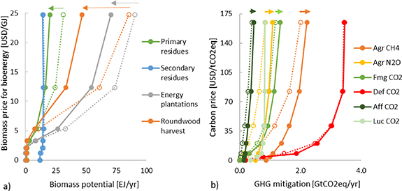
Figure 1. (a) Global biomass potential for bioenergy by feedstock in EJ yr−1 in 2050 without carbon price. Biomass prices represent USD GJ−1 primary biomass used for bioenergy. (b) AFOLU marginal abatement cost curves in GtCO2eq yr−1 in 2050 at baseline bioenergy levels. Solid lines—considering SDGs, dotted lines—not considering SDGs (noSDGs). Agr CH4 (methane from rice cultivation, enteric fermentation, and manure management), Agr N2O (nitrous oxide emissions from synthetic fertilizer and manure application, manure dropped on pastures, and manure management), Fmg CO2 (carbon dioxide emissions/removals from forest management), Aff CO2 (carbon dioxide emissions/removals from afforestation), Def CO2 (carbon dioxide emissions from deforestation), Luc CO2 (carbon dioxide emissions/removals from other land use changes).
Download figure:
Standard imageHigh-resolution image
Setting the estimated SDG compliant biomass potentials for bioenergy into perspective with existing 1.5 °C climate stabilization scenarios that anticipate an increase in biomass demand for bioenergy to 100–260 EJ by 2050 for SSP2 (Rogelj et al 2018), our results highlight a potential conflict between biodiversity conservation and scenarios with biomass deployment beyond 170 EJ yr−1. More stringent biodiversity protection schemes would even further exacerbate this trade-off. For example, if the AICHI target 11 that aims to increase protected areas to 17% by 2020 were doubled and one third of the global land surface were put under protection as suggested by the U.N. Convention on Biological Diversity in their draft plan for the post 2020 period, 4 biomass potentials could be limited to 130 EJ yr−1 only by 2050 (see supplementary material, figure S10 (stacks.iop.org/ERL/16/024006/mmedia)).
3.2. SDG compatible GHG mitigation potentials
SDGs are found to have positive synergies for AFOLU GHG abatement and to consistently decrease GHG emissions for both agriculture and forestry. Considering selected SDGs allows to reduce direct AFOLU emissions even in the absence of any mitigation efforts in the baseline scenario by 2.1 GtCO2eq yr−1 (1.4 GtCO2eq yr−1 from agriculture, and 0.7 GtCO2eq yr−1 from land use changes) in 2050. This is mainly driven by the decreased consumption of animal products, less food waste, and biodiversity protection which results in reduction of agricultural non-CO2 emissions from livestock and reduced CO2 emissions from land use change.
At 165 USD tCO2eq−1, a carbon price broadly in line with staying on track for the 1.5 °C target by 2050 (Rogelj et al 2018), AFOLU emission savings of up to 9.4 GtCO2eq yr−1 can be realized in 2050 as compared to the baseline without carbon prices and SDGs (figure 1(b). Reducing CO2 emissions, i.e. from deforestation, is an important low-cost mitigation option providing 40% of the mitigation at carbon prices <100 USD tCO2eq−1, while mitigation of agricultural non-CO2 emissions becomes increasingly important when moving towards higher carbon prices. Still, two thirds of the mitigation potential at 165 USD tCO2eq−1 can be attributed at global scale to the mitigation of CO2 emissions and the sequestration of carbon in managed and newly established forests.
However, the marginal impact of SDGs on the mitigation potential as compared to the noSDGs carbon price scenario is with additional 0.5 GtCO2eq yr−1 at 165 USD tCO2eq−1 rather small. This is because part of the agricultural mitigation potential when considering SDGs is already realized through the diet shift which leaves more limited scope for additional non-CO2 emission reduction at higher GHG prices as compared to the noSDGs variant. Hence, mitigation potentials tend to converge between SDG and noSDGs set-up with increasing carbon prices.
3.3. SDG compatible combined land-based mitigation potentials
Besides the adoption of SDGs, the level of biomass supply for bioenergy also significantly impacts, however in opposing directions, AFOLU emissions and the land use sector’s ability for GHG abatement (figure 2). With increasing levels of biomass supply for bioenergy, the AFOLU marginal abatement cost curve is shifted downward. While the carbon sink from the establishment of dedicated energy plantations increases and deforestation is reduced, these developments are overcompensated by a drop in the forest management sink through increased forest harvest for bioenergy and slightly reduced afforestation levels due to the increased competition for land. These effects are more pronounced in the scenarios without consideration of SDGs, whereas effects are less visible in the SDG scenarios where biodiversity protection limits the conversion of highly biodiverse primary forests and hence the negative impact on the forest carbon sink. Since GHG mitigation and bioenergy potentials are closely tied and interdependent as shown in figure 2, these interactions need to be considered in any land-based mitigation assessment.
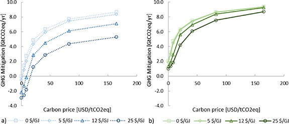
Figure 2. Impact of bioenergy prices on AFOLU mitigation potentials in GtCO2eq yr−1 in 2050 (a) without and (b) and with SDGs.
Download figure:
Standard imageHigh-resolution image
Looking at cumulative emissions in the baseline scenarios, achieving SDGs yields cumulative emissions savings of around 45 GtCO2eq by 2050 compared to the noSDGs baseline and even around 200 GtCO2eq until the end of the century. Putting these emissions savings into perspective with the cumulative AFOLU GHG abatement requirements projected by IAMs to stay on track with the 1.5 °C target by 2050 (Rogelj et al 2018), SDGs allow to realize already 25% of the expected cumulative AFOLU contribution (180 GtCO2eq mitigation by 2050) and even 40% of the expected cumulative contribution of 540 GtCO2eq by 2100.
SDG induced AFOLU emission reductions can be as high as 4 GtCO2eq yr−1 in 2050 (one third related to agriculture and two thirds related to forestry) when SDGs are combined with a biomass-based bioenergy mitigation strategy (biomass price for bioenergy of 25 USD GJ−1by 2050). Synergies with forestry and land use change emission reductions are most pronounced at high biomass prices related to protection of highly biodiverse primary forests. In total this could provide cumulative AFOLU emission reductions of up to 95 GtCO2eq by 2050 (285 GtCO2eq by 2100) (red area figure 3).
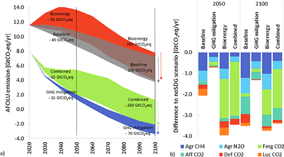
Figure 3. (a) Change in AFOLU emissions between SDGs and noSDGs scenarios for the baseline (no mitigation), bioenergy, GHG mitigation, and combined (bioenergy & GHG mitigation) scenarios over time. Grey area and arrow indicate the change when including selected SDGs in the baseline scenario without mitigation. Red area and arrow indicate the effect of including selected SDGs in a high bioenergy scenario (biomass price for bioenergy of 25 USD GJ−1 by 2050). Blue area and arrow indicate the effect of considering selected SDGs in a GHG mitigation scenario (GHG price of 165 USD/tCO2eq by 2050). Green area and arrow indicate the effect of considering selected SDGs in a combined bioenergy and GHG mitigation scenario (biomass price for bioenergy of 25 USD GJ−1 and GHG price of 165 USD tCO2eq−1 by 2050). The displayed numerical values represent changes in total cumulative AFOLU emissions from 2020–2050/2100 compared to the corresponding noSDGs scenario. b) Change in AFOLU emissions by GHG source between SDG and noSDGs scenarios in 2050 and 2100. Agr CH4 (methane from rice cultivation, enteric fermentation, and manure management), Agr N2O (nitrous oxide emissions from synthetic fertilizer and manure application, manure dropped on pastures, and manure management), Fmg CO2 (carbon dioxide emissions/removals from forest management), Aff CO2 (carbon dioxide emissions/removals from afforestation), Def CO2 (carbon dioxide emissions from deforestation), Luc CO2 (carbon dioxide emissions/removals from other land use changes).
Download figure:
Standard imageHigh-resolution image
However, reduced biomass availability for bioenergy affects mitigation potentials in the energy sector for bioenergy with carbon capture and storage (BECCs). To approximate the reduced emission reduction potential from BECCs (that would need to be compensated by other technologies) we use a back-of-the-envelope calculation. We assume a BECCs deployment rate of 60% in 2050 and a carbon sequestration efficiency of 0.07 GtCO2EJ−1 primary biomass based on the IAM results for the 1.5 °C pathway in SSP2 (Rogelj et al 2018). The calculated carbon sequestration efficiency which accounts only for the capture and storage of emissions from biomass burning is at the higher end as compared to other studies (Fajardy and Mac Dowell 2017, Fuss et al 2018) since other emissions i.e. from land use changes, are already accounted for in the presented AFOLU potentials. We find that the SDG induced biomass reduction at a biomass price for bioenergy of 25 USD GJ−1could translate into reduced BECCs mitigation of around 3.2 GtCO2 yr−1 by 2050 if BECCs is not substituted by other mitigation technologies. Though other studies have shown the feasibility of replacing BECCs with other mitigation technologies in the energy sector for example through behavioural change, while still achieving the 1.5 °C target (Grubler et al 2018, van Vuuren et al 2018), reduced biomass availability for bioenergy could increase the costs of climate change mitigation (Bauer et al, 2018, Calvin et al 2014, Muratori et al 2016).
Considering SDGs together with both bioenergy deployment and GHG mitigation allows to reduce AFOLU emissions by additional 3.4 GtCO2eq yr−1 by 2050 bringing down total AFOLU emissions to only 2 GtCO2eq yr−1 in 2050. Hence, SDGs allow for deeper and faster AFOLU emission cuts as compared to the noSDGs set-up. SDG induced cumulative GHG abatement amounts to around 65 GtCO2eq by 2050 (250 GtCO2eq until 2100) which represents already one third of the expected AFOLU GHG mitigation needed to stay on track with the 1.5 °C target. Results show that when considering SDGs, a 1.5 °C land use emission pathway could already be realized at 50 USD tCO2eq−1 by 2050, compared to 165 USD tCO2eq−1 in Rogelj et al (2018).
3.4. SDG compatible regional mitigation potentials
Having analysed global bioenergy and GHG mitigation potentials, their interdependencies and impact of selected SDGs, we want to bring down global potentials to the regional level. Across world regions, results show that Sub-Saharan Africa (around 50 EJ yr−1) followed by Latin America, Asia and OECD (each around 40 EJ yr−1) offer significant sustainable biomass potentials at 25 USD GJ−1and 165 USD tCO2eq−1 by 2050 without violating selected SDGs (figure 4). Overall, the regional distribution of the potentials is within the ranges estimated by other studies (Beringer et al 2011, Schueler et al 2013, Wu et al 2019). Even though absolute biomass potentials are similar across world regions, the underlying feedstock mix substantially differs (see supplementary material, Figure S11). For example, while in Latin America around half of the biomass for bioenergy is projected to be sourced from dedicated energy plantations, forests contribute two thirds in OECD countries and even three quarters of the biomass potential in Sub-Saharan Africa at 25 USD GJ−1and 165 USD tCO2eq−1. Looking at GHG mitigation potentials in the SDG scenarios, a more distinct picture arises across regions. Here, Latin America (3.3 GtCO2eq yr−1) and Asia (2.7 GtCO2eq yr−1) offer the highest abatement potentials at 25 USD GJ−1and 165 USD tCO2eq−1, followed by Africa and OECD with around 1.3 GtCO2eq yr−1 each.
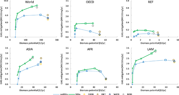
Figure 4. Regional GHG mitigation potentials conditional on the biomass potential in the noSDGs and SDG scenarios in 2050. Markers represent combinations of bioenergy and carbon prices 0 USD GJ−1and USD tCO2eq−1 (+), 2 USD GJ−1and 8 USD tCO2eq−1 (x), 3 USD GJ−1and 21 USD tCO2eq−1 (◊), 5 USD GJ−1and 41 USD tCO2eq−1 (△), 12 USD GJ−1and 82 USD tCO2eq−1 (□), and 25 USD GJ−1and 165 USD tCO2eq−1 (o). For 25 USD GJ−1and 165 USD tCO2eq−1 also additional points for individual SDGs (FOOD—food security, DIET—diet shift and food waste reduction, WATR—irrigation water, and BIOD—biodiversity protection) are displayed. OECD—North America, Europe, Pacific OECD; REF—Russia, Ukraine and Former Soviet Union; ASIA—South, East, and South-East Asia; AFR—Middle East and Africa; LAM—Latin and Central America.
Download figure:
Standard imageHigh-resolution image
Interestingly, several regional GHG abatement curves in figure 4 are slightly bent especially in the noSDGs scenarios which indicate that moving towards higher bioenergy supply results in decreasing mitigation potentials due to more intensive forest harvest beyond a certain point. While the aggregated AFOLU GHG abatement curve for OECD, African, and Former Soviet Union countries shows some saturation effect already beyond carbon prices of 40 USD tCO2eq−1 and biomass prices of 5 USD GJ−1, GHG mitigation potentials continue to increase in Asia and Latin America. This is related to the higher deployment of dedicated energy plantations in those regions instead of direct energy roundwood harvest from managed forests (see supplementary figure S11). Considering biodiversity protection is also shown to help to ease this trade-off, especially in combination with diet shift and reduced food waste. Hence, when considering SDGs, regional GHG abatement curves are much steeper as compared to the noSDGs scenarios. Overall, for all regions except the Former Soviet Union countries, the steep slope at the beginning of the curve hints that direct AFOLU emission reductions is a viable mitigation option at low (carbon and biomass) prices while biomass supply for bioenergy is becoming important when moving towards higher prices.
This study attempts to provide a comprehensive model-based assessment of capacity of the AFOLU sector to contribute to ambitious climate change mitigation within the SDG agenda. Considering selected SDGs, in particular protecting highly biodiverse ecosystems from conversion, was shown to substantially reduce global biomass potentials for bioenergy to 170 EJ (−30%) in 2050. The analysis indicates that the protection of highly biodiverse areas is, depending on the level of ambition, the key limiting factor for biomass availability for energy use. For example, doubling the efforts of the AICHI target 11 and protecting around one third of the world surface would further decrease biomass availability for bioenergy to around 130 EJ in 2050. Similarly, Erb et al (2012) projected a reduction in the global bioenergy potential by 9%–32% depending on the ambition of conservation efforts and Wu et al (2019) estimate a sustainable biomass potential of around 150 EJ globally. Given likely trade-offs between land-based bioenergy deployment and biodiversity (Santangeli et al 2016, Heck et al 2018, Hof et al 2018), there remains a need to reconcile current 1.5 °C climate stabilization pathways with substantial BECCs and SDG15—Life on Land, which in itself poses a huge and complex challenge (IUFRO 2019, Leclère et al 2020). Energy demand side transformations could provide a viable contribution and enable climate stabilization with very limited additional biomass demand for bioenergy (Grubler et al 2018, van Vuuren et al 2018). In addition, enhanced conservation and restoration measures accompanied by cross-sectorial measures to realize synergies with other SDGs are indispensable to reverse the continued biodiversity loss from habitat conversion (IUFRO 2019, Leclère et al 2020).
We show that SDGs, GHG mitigation and biomass potentials are strongly interdependent and need to be systematically assessed together. We estimate that even in the absence of targeted mitigation efforts in the land sector, achieving SDGs could drive emissions reductions from land use of 2.1 GtCO2eq yr−1 in 2050 related to reduced consumption of ruminant products and food waste (1.4 GtCO2eq yr−1) as well as biodiversity protection and related decline in land use change emissions (0.7 GtCO2eq yr−1). Likewise other studies estimated an agricultural non-CO2 mitigation potential between 0.7–3.3 GtCO2eq yr−1 in 2050 induced by a shift towards healthy diets (Stefan Springmann et al 2016, Frank et al 2019) and highlight potential synergies between biodiversity conservation and GHG mitigation (Strassburg et al 2012, Bernardo B N Strassburg et al, 2019, Jung et al 2020).
Achieving the assessed SDGs would allow to realize cumulative GHG abatement of 45 GtCO2eq by 2050. This alone represents already 25% of the expected AFOLU abatement requirements until 2050 projected by IAMs to stay on track with the 1.5 °C target (Rogelj et al 2018). By the end of the century, SDGs could allow to even deliver 40% of the expected contribution from the land use sector according to IAMs thereby reducing the land use related mitigation costs substantially. If SDGs and climate change mitigation efforts are pursued jointly, this strengthens synergies further. Results show that SDGs allow for even more rapid and deeper emissions cuts as compared to the scenarios without consideration of SDGs. AFOLU emissions could drop to 2 GtCO2eq yr−1 in 2050 thereby delivering emission savings of around 8.7 GtCO2eq yr−1 as compared to a baseline without mitigation efforts in 2050 (at 165 USD tCO2eq−1 and a biomass price for bioenergy of 25 USD GJ−1). Hence, considering SDGs could allow the land use sector to remain within a 1.5 °C compatible land use emission budget of 275 GtCO2eq by 2050 (Rogelj et al 2018) already at only 50 USD tCO2eq−1, however, without considering opportunity costs in other economic sectors aside agriculture and forestry which could increase abatement costs.
The estimated AFOLU mitigation potentials are in line with other modelling studies (Popp et al, 2017, Rogelj et al 2018, Roe et al 2019) but slightly more conservative as compared to bottom–up estimates by Griscom et al (2017). For example, Griscom et al (2017) estimate a AFOLU mitigation potential of around 11.3 GtCO2eq in 2030 at 100 USD tCO2eq−1, 7.3 GtCO2eq from forests, 2.5 GtCO2eq from agriculture and 1.5 GtCO2eq from wetlands. Main reasons for the difference are missing representation of mitigation from wetlands and agricultural soil organic carbon in our study as well as the absence of dynamic interactions and interdependencies between the land-based mitigation options in Griscom et al (2017). The estimated sustainable biomass potentials are within the ranges with high agreement (100–300 EJ) based on a literature review by Creutzig et al (2015). Similarly Wu et al (2019) show that biomass potentials could drop from 245 EJ to 160 EJ when considering biodiversity protection.
In combination with efforts to enhance food production and food security more competition for land and hence more limited scope for land-based mitigation could be anticipated. On the contrary, biomass and mitigation potentials could be underestimated as mitigation from wetlands and soil organic carbon in agriculture (up to 3 GtCO2eq yr−1 at 100 USD tCO2eq−1 (Griscom et al 2017)) or biomass potentials from agricultural residues (10–66 EJ (Slade et al 2014)) are not included in the analysis. Besides, only a subset of sustainability indicators and SDG targets were explicitly assessed. Extending the analysis, for example accounting for temporal lags in land system change (Brown et al 2019) but also to encompass a more detailed welfare assessment across economic sectors and actors using Computable General Equilibrium models (Golub et al 2013, Hussein et al 2013, Tabeau et al 2017) would further improve robustness of results. For example, Golub et al (2013) positive welfare effects of land-based mitigation policies for farm households while unskilled urban households typically experience welfare losses without accompanying policies.
The next round of assessments should therefore move from integrated assessment of climate stabilization pathways towards testing feasible policy instruments that can be applied by decision makers at national/regional scale. Accompanied with comprehensive ex-post monitoring along multiple sustainability dimensions, this would not only allow to develop pathways but actually guide and monitor the transformation of the land use sector towards climate stabilization (Brown et al 2019). Like—albeit the above mentioned needs for further research, this study provides a comprehensive assessment of synergies and trade-offs between mitigation strategies in the land use sector in the context of SDGs, and a useful dataset which will enhance future integrated assessments.
The data that support the findings of this study are openly available at the following URL: https://github.com/iiasa/GLOBIOM-G4M_LookupTable.
This study has been funded by the Joint Research Centre of the European Commission through the RepLandusePattern project (contract number 931609-2016 A08-AT), the European Union’s H2020 CD-LINKS (grant agreement no. 64214), ENGAGE (grant agreement no. 821471), NAVIGATE (grant agreement no. 821124) and Directorate General Climate Action (EC Service contract N°340201/2015/717962/SERJCLIMA.A4). The authors also acknowledge the Global Environment Facility (GEF) for funding the development of this research as a part of the ‘Integrated Solutions for Water, Energy, and Land (ISWEL)’ project (GEF contract agreement: 6993).
The authors declare no competing interests.
SF and PH designed the research and performed the scenario development supported by TH (undernourishment), AP (water), and HV (diets). Simulations were carried out by SF (GLOBIOM) and MG (G4M). SF performed first analysis of the results, produced the figures, and led the writing of the paper in collaboration the other authors. All authors provided feedback and contributed to the discussion and interpretation of the results.