Rapid decline in carbon monoxide emissions and export from East Asia between years 2005 and 2016 (original) (raw)
1748-9326/13/4/044007
Abstract
Measurements of Pollution in the Troposphere (MOPITT) satellite and ground-based carbon monoxide (CO) measurements both suggest a widespread downward trend in CO concentrations over East Asia during the period 2005–2016. This negative trend is inconsistent with global bottom-up inventories of CO emissions, which show a small increase or stable emissions in this region. We try to reconcile the observed CO trend with emission inventories using an atmospheric inversion of the MOPITT CO data that estimates emissions from primary sources, secondary production, and chemical sinks of CO. The atmospheric inversion indicates a ~ −2% yr−1 decrease in emissions from primary sources in East Asia from 2005–2016. The decreasing emissions are mainly caused by source reductions in China. The regional MEIC inventory for China is the only bottom up estimate consistent with the inversion-diagnosed decrease of CO emissions. According to the MEIC data, decreasing CO emissions from four main sectors (iron and steel industries, residential sources, gasoline-powered vehicles, and construction materials industries) in China explain 76% of the inversion-based trend of East Asian CO emissions. This result suggests that global inventories underestimate the recent decrease of CO emission factors in China which occurred despite increasing consumption of carbon-based fuels, and is driven by rapid technological changes with improved combustion efficiency and emission control measures.
Export citation and abstractBibTeXRIS
Carbon monoxide (CO) is produced by the incomplete combustion of carbon-based fuels and atmospheric oxidation of hydrocarbons. It is the dominant sink of the hydroxyl radical (OH), which controls the oxidizing power of the troposphere, and hence influences the lifetime of most atmospheric pollutants and reactive greenhouse gases. Each reaction of CO with OH radicals has a theoretical maximum yield of one ozone (O3) and one carbon dioxide (CO2) molecule, which results in an indirect positive radiative forcing around 0.2 W m−2 (Myhre et al 2013).
The Measurements of Pollution in the Troposphere (MOPITT) space-borne instrument has been measuring tropospheric CO since 2000, and shows a decreasing global trend ~ −1% yr−1 in CO total column, with stronger trends (−1.42 to −1.60% yr−1) identified over Europe, the United States, and East Asia for 2000–2010 (Worden et al 2013). Measurements of surface concentrations confirm similar declining trends (Yoon and Pozzer 2014). The reduction of CO pollution is consistent with bottom-up emission inventories indicating reduced emissions in Europe and the United States, and chemical transport model simulations driven by those inventories reproduce the negative trends of observed CO concentrations (Yoon and Pozzer 2014, Strode et al 2016). This suggests that emission inventories over these two regions successfully track the progress of emission reduction due to pollution control.
However, global inventory data show increasing emissions over East Asia, which cannot be reconciled with observed CO concentrations (Strode et al 2016). A downward trend ~ −1.6% yr−1 in CO concentrations is observed by MOPITT (Worden et al 2013) over East Asia for years 2000–2010, but model simulations using the time-dependent MACCity inventory (Granier et al 2011) show upward trends. Strode et al (2016) analyzed possible model biases that contributed to the model-observation discrepancy, and found that an overestimate of O3 associated with less O3 break-up forming less OH played an important role. While chemistry model biases examined by Strode et al (2016) cannot explain all aspects of the inconsistencies, their study also questioned the increasing CO emission trends of the MACCity inventory. Yet other global bottom-up inventories also show increasing CO emissions (0.9%–2.9% yr−1) from East Asia over the past decade (Granier et al 2011, Crippa et al 2016, Zhong et al 2017). Anthropogenic sources are the major sources of CO in East Asia. The increasing emissions from East Asia reported by global bottom-up inventories are mainly caused by growing anthropogenic sources, which include industrial boilers, residential stoves, iron and steel production, and motor vehicles. Conversely, top-down atmospheric inversion-based emission estimates assimilating CO observations (Tohjima et al 2014, Yumimoto et al 2014, Yin et al 2015, Jiang et al 2017) all yield negative CO emission trends (−2.0 to −3.2% yr−1, for 2005–2015), though the inversion approach cannot attribute the driving forces.
In the present study, we reevaluate the 2005–2016 trends of CO concentrations over East Asia, and analyze the underlying drivers of CO changes. Here East Asia refers to the geographical area covering Mainland China, Hong Kong, Macau, Taiwan, Japan, Mongolia, North Korea, and South Korea. Our goal is to understand the inconsistencies between observed and modeled CO trends over East Asia reported by previous studies. We first investigate the tropospheric CO column from the MOPITT version 7 product (Deeter et al 2017). Then, we use a Bayesian inversion technique (Chevallier et al 2005) jointly assimilating observations of the main species involved in the oxidation chain of hydrocarbons to estimate the sources and sinks of atmospheric CO. Both the diversity of assimilated data and the treatment of the uncertainty in CO chemical production and sinks are important features of our method that permit the reliable estimation of the trends in CO emissions over East Asia.
Below, we first describe the tools used to analyze the sources and sinks of atmospheric CO: the MOPITT satellite measurements, the atmospheric inversion model that assimilates these data to provide optimized surface CO emissions, secondary CO production, and CO destruction by OH in the atmosphere, and the inventories used for comparison with inversion emissions. Then the observed trends in MOPITT data are analyzed, inversion CO emissions trends are discussed and compared with inventories.
We show that the declining trend in CO concentrations over East Asia of −0.41 ± 0.09% yr−1 for 2005–2016 (P < 0.001, 95% confidence interval, two-tailed) can be explained by a −2.51 ± 0.94% yr−1 (P < 0.001) decrease in CO emissions from primary sources in this region, which outweighs increasing secondary CO production (1.56 ± 0.56% yr−1, P < 0.001) due to the rising CH4 concentrations and NMVOC emissions. Global bottom-up emission inventories fail to reproduce the negative trend of CO emissions probably because they underestimate the strength of emissions control in China, whereas the detailed inventory of Multi-resolution Emission Inventory for China (MEIC, www.meicmodel.org/) matches the top-down inversions well. The MEIC data is further analyzed to investigate sectors and emission factors that drive the decreasing CO emissions in China, which accounts for 84% of the CO emissions decrease during 2005–2016 in East Asia.
2.1. MOPITT Version 7 CO
The MOPITT instrument was launched aboard the EOS-Terra satellite platform in December 1999 and began reporting data in March 2000 (Deeter et al 2003). It measures CO column on the global scale, which means the number of CO molecules between the MOPITT instrument and the Earth’s surface per area of the surface (i.e. molecules cm−2). The MOPITT retrieval products have been improved continuously, as confirmed by independent validation data, since 2000. Retrieval product improvements are the result of radiative transfer model enhancements, updated a priori information, and bias corrections (Deeter et al 2010, 2013, 2014).
In this study, we use MOPITT Version 7 (V7) level 2 total column retrievals from the multispectral TIR-NIR product. First V7 products were released in August 2016. As demonstrated by comparisons with CO in-situ vertical profiles measured from aircraft over North America, MOPITT V7 products exhibit much improved error characteristics (Deeter et al 2017). In contrast with the previous V6 product, for example, the overall biases for V7 are a few percent or less at all levels for the TIR-only, NIR-only and TIR-NIR products. For the period from 2000–2015, analysis of the long-term bias trends (i.e. bias drift) for the V7 TIR-NIR product indicates a negative bias drift for the lower-troposphere (e.g. −1.04% yr−1 at 800 hPa) and an opposing positive bias drift for upper-tropospheric retrieval levels (e.g. 1.15% yr−1 at 400 hPa). However, due to the opposite effects of bias drift in the lower and upper troposphere, the reported bias drift for the TIR-NIR total column product is nearly negligible (e.g. a relative bias drift of less than 0.1% yr−1, thus much smaller than the CO trend in East Asia). To exclude retrievals with low information content, we use only satellite retrievals with solar zenith angle less than 70°, surface pressure greater than 900 hPa, and latitude within 65°S–65°N (Fortems-Cheiney et al 2011, Yin et al 2015).
2.2. Atmospheric inversion
We use a variational Bayesian approach (Chevallier et al 2005) to estimate CO emissions from primary sources, secondary production, and chemical sinks of CO for 2005–2016 (detailed in text S2–7). Technically, the Bayesian inference can be solved as a variational optimization problem by minimizing the following cost function:
The variables that we seek to estimate are assembled into the state vector x. Through optimization we obtain the optimal x given a priori guess xb and observation vector y, for which the error statistics are represented by covariance matrices B and R, respectively. x and y relate to each other through the forward model H that can be simply understood as an operator calculating y as a function of x. In this study, the Bayesian framework is used in the hydrocarbon oxidation chain, consisting of methane (CH4), formaldehyde (HCHO), CO, CO2 as well as intermediate species, with chain reactions driven by OH among all chemical species (Pison et al 2009). Methyl chloroform (MCF) is also included to constrain OH concentrations.
The state vector x contains OH concentrations, emission fluxes of CH4, HCHO, CO and MCF, and the initial concentration fields of these four species. The a priori CO sources include MACCity anthropogenic emissions (Granier et al 2011, downloaded from http://eccad.sedoo.fr), GFED 4s biomass burning emissions (van der Werf et al 2017, downloaded from www.globalfiredata.org/index.html), MEGAN biogenic emissions (Sindelarova et al 2014, downloaded from http://eccad.sedoo.fr), and POET oceanic emissions (Olivier et al 2003, Granier et al 2005, downloaded from http://eccad.sedoo.fr). These datasets are selected as a priori emissions input because they represent the most up-to-date period of CO emission fluxes freely available on global scales. The MACCity dataset is the only available dataset that provides monthly anthropogenic emissions that cover 2005–2016 (data after 2010 are emission projections). The GFED4s dataset is the latest data on biomass burning emissions that achieve high accuracy (van der Werf et al 2017), and the MEGAN and POET dataset are both the latest emissions data. The a priori information for the other variables and covariance matrix B follow the configurations of Yin et al (2015, 2016).
The observation vector y consists of satellite CO and HCHO tropospheric columns, and surface concentrations of CH4 and MCF from in-situ networks. We use CO column retrievals from the MOPITT V7 product (Deeter et al 2017), HCHO column retrievals from the Ozone Monitoring Instrument V003 product (González et al 2015), CH4 and MCF surface air-sample measurements from the World Data Centre for Greenhouse Gases dataset (WDCGG, http://ds.data.jma.go.jp/gmd/wdcgg/). The forward model H is LMDz-SACS (1.9° lat × 3.75° lon × 39 vertical layers), a 3D transport model with a simplified chemistry scheme. LMDz is a general circulation model (http://lmdz.lmd.jussieu.fr/) which is nudged towards the European Centre for Medium-Range Weather Forecasts analyses for horizontal winds. The LMDz model is coupled with SACS module, a simplified chemistry module for the oxidation chain of hydrocarbons, which is developed by Pison et al (2009) on the basis of the Interaction with Chemistry and Aerosols (INCA) full chemistry model (Hauglustaine et al 2004). The LMDz-SACS model is described in Text S2. Details of y, H and covariance matrix R refer to Yin et al (2015, 2016).
The inversion solves for emission fluxes of CH4, CO and MCF in each surface grid cell (1.9° lat × 3.75° lon) of the transport model over eight day periods (detailed in Text S3). This inversion system has been much used and evaluated in the optimization for sources of CH4, CO and HCHO at both global and regional scales (Chevallier et al 2009, Pison et al 2009, Fortems-Cheiney et al 2009, 2011, 2012, Yin et al 2015, 2016). We also collected emission estimates from two regional inversion systems including China for comparison. They are from Tohjima et al (2014) (assimilating surface observations for 1999–2010) and Yumimoto et al (2014) (assimilating MOPITT Version 5 data for 2005–2010).
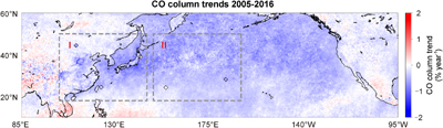
Figure 1. Tropospheric CO column trends derived from MOPITT V7 data over 0.5° × 0.5° grid cells. Time series of 2005–2016 data are analyzed using a curve fitting method (text S1 available at stacks.iop.org/ERL/13/044007/mmedia) to calculate the CO column trends. The diamonds represent the six WDCGG sites used for trend analysis of CO surface concentrations.
Download figure:
Standard imageHigh-resolution image
2.3. Bottom-up inventories
We use a regional emission inventory, the MEIC version 1.2 data (www.meicmodel.org/), to analyze the drivers of long-run CO emissions in China, which represents 90% of East Asian CO emissions. The MEIC model is a technology-based emission inventory framework developed by Tsinghua University (Zheng et al 2014, Liu et al 2015). The main emission sources are identified and quantified through the product of activity data and time-dependent emission factors, which are estimated by technology turnover models that track the penetration of different combustion technology used in emission source sectors. As emissions rates depend on combustion technology, this method can calculate dynamic emission factors that reflect technological changes over time (Zhang et al 2009, Lei et al 2011, Liu et al 2015). The MEIC database provides time series of emission estimates for China spanning from 1990–2015. We use MEIC sectoral changes of CO emissions to investigate the drivers behind the variations of inversion-based emissions. To compare with the MEIC data and our inversion results, we also collected data from six bottom-up inventories including PKU (2005–2014) (Zhong et al 2017), REAS v2.1 (2005–2008) (Kurokawa et al 2013), EDGAR v4.3 (2005–2010) (Crippa et al 2016), MIX (2006, 2008 and 2010) (Li et al 2017), and the data from Xia et al (2016) (2005–2014) and Zhao et al (2012) (2005–2009).
MOPITT observes a substantial decrease in tropospheric CO column over East Asia from 2005–2016 (figure 1). Geographically, the pattern of decreasing linear trends fitted to the data is not evenly distributed. Western China that is generally upwind of the heavily industrialized areas of China to the east, presents relatively weak CO trends. Larger decreases generally occur in industrialized areas with higher CO levels, such as in eastern China (−1 to −2% yr−1). MOPITT also observes a strong decrease in CO (~ −1% yr−1) off the coast of East Asia (figure 1, box II), and similar decreases over the eastern Pacific, suggestive of reduced export of CO from East Asia via the prevailing westerlies.
Monthly average observations reveal the detailed temporal evolution of CO column (blue curves in figures 2(a) and (b)). The peak column CO in winter/ spring shows a large, significant decrease (P = 0.003) of −0.54 ± 0.31% yr−1 over East Asia (figure 1, box I), while that in summer/fall exhibits a small, insignificant decrease (P = 0.131) of −0.33 ± 0.45% yr−1. The de-seasonalized monthly CO column shows a medium, significant decrease (P < 0.001) of −0.41 ± 0.09% yr−1 (blue curves in figure 2(c)). The downwind oceanic region of East Asian continent (figure 1, box II) exhibits similar decreasing linear trends (blue curves in figures 2(b) and (d)). We also investigate surface concentrations of CO from the WDCGG dataset, which includes six remote observing stations (the diamonds in figure 1) within East Asia and its downwind areas. De-seasonalized monthly surface observations show a significant negative trend (P < 0.001) of −0.46 ± 0.14% yr−1 for 2005–2016, driven by a significant decrease (P = 0.008) of −1.00 ± 0.67% yr−1 in winter/spring. The observed decrease of mean annual surface concentrations (−0.46 ± 0.14% yr−1, P < 0.001) is similar to the linear trend of CO column (−0.41 ± 0.09% yr−1, P < 0.001) observed by MOPITT. We note that the time period selected for the trend calculation is also important due to significant variability in global CO from large biomass burning episodes such as the boreal fires in 2002, 2003 (Yurganov et al 2005) and the El Nino driven fires in Indonesia in September–October 2015 (Field et al 2016, Yin et al 2016).
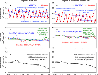
Figure 2. 2005–2016 observed and simulated changes in monthly CO column over East Asia (a), (c) and (e) and the downwind oceanic area (b), (d) and (f). The blue curves represent MOPITT CO time series (a) and (b) and its trend data (c) and (d), and red curves are for LMDz-SACS simulations with optimized emissions (a) and (b) as well as its trend data (c) and (d). The green curves represent the trend data of sensitivity simulation with primary CO emissions of East Asian countries (China, Mongolia, North Korea, South Korea, and Japan) held constant at the levels of year 2005 (c) and (d). The effects of East Asian CO emissions change on the trends in MOPITT CO observations (black curves in (e) and (f)) are estimated as the 2005–2016 emissions run (red curves in (c) and (d)) minus 2005 constant emissions run (green curves in (c) and (d)). The trend data (c)–(f) are calculated using the curve fitting method that is described in text S1.
Download figure:
Standard imageHigh-resolution image
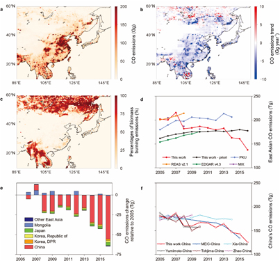
Figure 3. CO emissions for 2005–2016 estimated by the inversion. The emission map of 2005 (a) are downscaled from 1.9° × 3.75° to 0.5° × 0.5° following the spatial pattern of a priori emission fluxes in the same large grid. Emission trends (b) are represented by the slope of linear regression lines through annual emissions between 2005 and 2016. Percentages of biomass burning emissions averaged for 2005–2016 (c) are derived from the a priori emission fluxes. We review previous studies on CO emissions trends over East Asia (d) and China (f), and compare them with our inversion results. (e) CO emission change relative to that of 2005 by country.
Download figure:
Standard imageHigh-resolution image
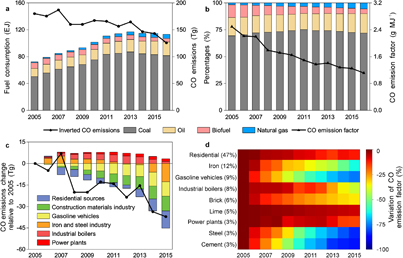
Figure 4. Driving forces of the declining CO emissions in China. (a) China’s energy consumptions by fuel type (bar charts) and the inversion CO emissions (black curve). (b) China’s fuel mix (stacked bar charts) and the average emission factor of CO on fuel base (black curve). (c) Comparison of CO emissions change relative to 2005 derived from the MEIC data (by source sector, bar charts) and that derived from the inversion results (black curve). The construction materials industry includes the industries of brick, lime, and cement. (d) Changes of CO emission factors with respect to the year 2005 by source in China. The numbers with brackets displayed along the y axis represent the emission shares of 2015 estimated using the MEIC data.
Download figure:
Standard imageHigh-resolution image
The results from the LMDz-SACS inversion assimilating MOPITT CO and other related tracer measurement show a linear reduction of −2000 to −4000 kg km−2 yr−1 in high emission areas such as East China, South Korea and Japan for 2005–2016 (figures 3(a) and (b)). The anthropogenic sources drive the downward trend because biomass burning contributes less (figure 3(c)). We also see a linear growth of < 2000 kg km−2 yr−1 in CO emissions over the areas adjacent to South Central Siberia due to increased fire activities (figures 3(b) and (c)). However, compared with the widespread decline in emissions over high emission areas, the slight increase of wildfires has little effect on net emissions due to their small size.
Inversion-based estimates show a decreasing trend of −2.51 ± 0.94% yr−1 for CO emissions in East Asia (P < 0.001) with respect to 2005 (−5.07 Tg year−1) spanning from 2005–2016 (the red solid curve in figure 3(d)). This negative trend is not present in the a priori emission fluxes used in the LMDz-SACS inversion (the black solid curve in figure 3(d)). For China specifically, the inversion infers a decrease of −2.16 ± 3.40% yr−1 (P = 0.152) for 2005–2010, which is close to the regional inversions of Tohjima et al (2014) and Yumimoto et al (2014) that show a linear emission decrease of ~−2% yr−1 in China for the same period. Overall, our inversion results for East Asia change in three successive phases: Phase I (2005–2007, a slight increase), Phase II (2008–2013, a drop by 15.55% in 2008 and then a slight decrease of −0.18 ± 0.91% yr−1, P = 0.621), and Phase III (2014–2016, an accelerated decline). The abrupt drop of CO emissions in 2008 is coincident with a sharp decrease in MOPITT CO column in the second half of this year (figure 2(c)) as reported by Witte et al (2009), Yurganov et al (2010), Worden et al (2012) and Strode et al (2016). Witte et al (2009) showed CO reductions of 12% at 700 hPa using the MOPITT data that was attributed to rapid and strict controls on pollutant emissions in East China for the Beijing Olympics in August–September 2008. Yurganov et al (2010) estimated that the upper limit of monthly drop of CO column could reach 30% at the end of 2008 due to reduced activities during the economic recession. Therefore, one may think that the abrupt drop of 2008 CO emissions over East Asia was probably caused by stringent pollution control for the Beijing Olympics followed by the subsequent sharp slowdown in the GDP growth and stalled industrial production.
In Phase I, the inversion-based emissions agree well with REAS v2.1 and MIX bottom-up inventories, and exhibit similar growth to other bottom-up inventories. In Phase II, our inversion emissions are consistent with the MIX data for the years of 2008 and 2010, but are distinct from the PKU data, MACCity data and EDGARv4.3. These three global inventories fail to reproduce both the large and abrupt fall of emissions in 2008 and the slight decrease after that. In Phase III, the inversion estimate of this work shows an accelerated decreasing trend in emissions, inconsistent with the rising emissions of MACCity. The global bottom-up inventories mentioned above fail to reflect the evolution of emissions over East Asia during Phases II and III, thus they cannot capture the declining CO trend for 2005–2016. Over all three phases, China is responsible for 84% of the decrease (the red bar in figure 3(e)), suggestive of the dominant role that China plays in the trend and variability of East Asian CO emissions.
We further evaluate the inversion emissions over China (the red curve in figure 3(f)) against the MEIC inventory (the blue curve in figure 3(f)). The MEIC data shows a decreasing linear trend of −2.16 ± 0.79% yr−1 (P < 0.001) which agrees well with our inversion estimates (−1.86 ± 0.92% yr−1, P = 0.001) for 2005–2015, while the bottom-up emission inventories developed by Xia et al (2016) and Zhao et al (2012) both show flattening emissions. Still, none of these regional bottom-up inventories can capture the abrupt drop of CO emissions in 2008.
We use the LMDz-SACS forward model to check the contributions of primary CO emissions trends (−2.51 ± 0.94% yr−1, P < 0.001) to the observed 2005–2016 trend of CO concentrations (−0.41 ± 0.09% yr−1, P < 0.001). Using the optimized emissions, optimized OH concentrations, and initial concentration fields inferred from the inversion, the forward model reproduces the absolute magnitude and temporal evolution of MOPITT observations well (red curves in figures 2(a)–(d)), indicating that the inversion fits the CO concentrations well.
To quantify the impacts of East Asian CO source change on the trends in MOPITT CO observations, we conduct a sensitivity simulation with primary CO emissions held constant at the levels of year 2005 in East Asian countries (green curves in figures 2(c) and (d)) and other factors—emissions in other regions, OH concentrations, and initial concentration fields—being variable and taken from the inversion. The modeling results for this sensitivity simulation show a positive, insignificant trend of CO column (0.03 ± 0.08% yr−1, P = 0.474) over East Asia (figure 2(c)), indicating that the other factors in the model do not explain the decrease of CO concentrations, and thus that only a reduction of primary CO emissions in East Asia can match the MOPITT trends (−0.41 ± 0.09% yr−1, P < 0.001). These results are consistent with the findings of Strode et al (2016), whose simulation with constant CO emissions showed a positive trend in CO concentrations for 2000–2010 over East China. Worden et al (2013) also suggests a decrease of primary CO emissions over East China to match the declining CO concentrations in this region for 2000–2011.
We subtract the model run driven by constant 2005 emissions from the simulation with variable 2005–2016 emissions (black curves in figures 2(e) and (f)). The 2005–2016 emission update results in a decrease of −0.42 ± 0.04% yr−1 (P < 0.001) in CO column (figure 2(e) that matches the MOPITT observations well (−0.41 ± 0.09% yr−1, P < 0.001, figure 2(c)). The same holds true in areas downwind (figures 2(d) and (f)). These results show that primary emissions change over East Asian countries can account for the entire declining trend of CO concentrations observed in this region.
As China dominates the East Asian emission budget, and because of the good match between inversion-based emission estimates and the independent bottom-up MEIC inventory, we use the MEIC data to understand the drivers behind the declining trends of Chinese emissions (figure 4). In MEIC, China’s CO emissions keep falling because decreasing emission factors totally offset the increasing use of carbon fuels (figures 4(a) and (b)). Generally, all important source sectors (e.g. residential, iron, gasoline-powered vehicles, and industrial boilers) are improving combustion efficiency and strengthening air pollution control in the last decade, which ultimately leads to the steady decline in emission factors spanning from −7% to −86% across sources for 2005–2015 (figures 4(c) and (d)).
Four source sectors dominate the downward trends of China’s emissions, including iron and steel industries, residential sources, gasoline-powered vehicles, and construction materials industries (figure 4(c)). These four sectors are responsible for 92% of China’s emissions cut, and can explain 76% of the emissions decrease for East Asia. In iron and steel industries, CO is an unavoidable byproduct released from blast furnace and basic oxygen furnace. Industry operators have reduced gas leaks, so the amount of CO emitted to the atmosphere is decreasing (−62% for iron production and −84% for steel making in 2005–2015 estimated by the MEIC data). Residential sources contribute half of CO emissions in China due to the extensive use of low-efficiency fuels and stoves. China has started to promote the use of clean stoves and phase out traditional biofuels (i.e. wood and crop residual) since 1990s (World Bank 2013), which helps lower CO emission rates of the residential sector (−12% for 2005–2015). The emissions from gasoline-powered vehicles are controlled successfully with the increasingly more stringent emission standards from stage 2 (equivalent to Euro 2/II standards) to stage 5 (equivalent to Euro 5/V standards) implemented since 2005 (Wu et al 2017). Consequently, the fleet average CO emission factor has been reduced by 76% from 2005–2015 according to the MEIC emission factors. The construction materials industries reduce emissions through using high efficiency kilns. For example, the cement industry replaces low-efficiency shaft kilns with a new type of rotary kiln, called the new dry process in China, in the last decade (Lei et al 2011). The percentage of cement produced by the new kilns increase from 44% in 2005 to 99% in 2015, which reduces the CO emission factor by 86%. These four sectors show a much larger decline of emissions since 2013, because China accelerated the air pollution control at the end of 2013 to fight against severe haze pollution (State Council of the People’s Republic of China 2013).
In this study, we have analyzed the main sources of inconsistency between 2005–2016 CO trends from MOPITT column observations and from global emission inventories in East Asia. The most important findings are that (1) the decreasing linear trend of −0.41 ± 0.09% yr−1 (P < 0.001) in CO concentrations over East Asia is due to a −2.51 ± 0.94% yr−1 (P < 0.001) decrease in emissions from primary sources in this region, that is a cumulative decline of −32% from 2005 to 2016 and (2) 76% of the emissions decline over East Asia can be explained by emissions control of four source sectors in China, i.e. iron and steel industries, residential sources, gasoline-powered vehicles, and construction materials industries. This emission decrease is enough to counterbalance the effect of rising concentrations of CH4 (0.38 ± 0.01% yr−1, derived from WDCGG observations) and increasing emissions of NMVOC (4.59 ± 0.44% yr−1, estimated by MEIC data) in East Asia, that increase the secondary CO formation at a rate of 1.56 ± 0.56% yr−1 (P < 0.001) according to our multispecies inversion (Text S7). Global bottom-up emission inventories were less successful in capturing the negative emission trends than the MEIC inventory, probably because they underestimate the strength of emissions control in East Asia, especially in China. The MACCity inventory since 2010 are emission projection data so they cannot reflect the recent trends in China CO emissions, and changes in emission factors. As a fast-growing economy with rapid technology changes, emission factors vary so fast that capturing the CO emissions variation remains a big challenge. Moreover, multi-instrument space-borne observations also verified recent (2005–2015) reductions in air pollution loadings of sulfur dioxide, nitrogen dioxide and aerosols over East Asia (Krotkov et al 2016, Liu et al 2016, Zhang et al 2017, Zhao et al 2017). It is difficult to predict these changes using models and conservative estimates. Our research method incorporating observations, inverse modeling and technology based bottom-up inventory provides an opportunity to better understand what happened recently as well as the underlying drivers. Though all data and methods are subject to their own uncertainties, the final results are considered robust given the consistency between observations from MOPITT satellite and ground-based CO measurements (section 3), between our inversion analysis and other inversion results (section 4), and between our inversion results and the latest bottom-up emissions data (section 5).
Data to support this research are available upon request to the corresponding author Bo Zheng (bo.zheng@lsce.ipsl.fr). We acknowledge the data providers of NCAR MOPITT for satellite CO retrievals, SAO OMI for CH2O retrievals, and WDCGG for CH4, CO, and MCF surface air-sample measurements. We also thank F Marabelle for computer support at LSCE.