Modelling developmental instability as the joint action of noise and stability: a Bayesian approach (original) (raw)
A simple model of DN, DS and DI
We assume that in the absence of a mechanism that buffers development against random noise, developmental errors will accumulate and result in a phenotype that deviates from its expected value given the individuals' genotype and environmental conditions. Each developmental mistake is assumed to be independent of previous ones and to follow a normal distribution with zero mean and variance equal to σ2 noise. It is important to note that these assumptions which also hold in previous models, may be an unrealistic oversimplification of real developmental processes [1, 13]. Representing development as a high number of small discrete growth events, any trait value is a sample from a normal distribution with mean equal to the expected trait value and variance the sum of the many small errors over a range of growth events:
The asymmetry of a bilaterally symmetric trait then follows:
N(0,DN) (2)
where developmental noise is defined as the cumulative effect of mistakes:

DS, the process that buffers development against mistakes, can be incorporated in this model as the proportional reduction in σ2 noise during development. Asymmetry of bilateral symmetric traits then follows:
N(0,DN × (1 - DS)) (3)
where DS ∈ [0,1[ and large values of DS indicate high buffering capacity. Note that 1 is not included in the domain of DS since this would lead to a zero variance. The model hereby assumes that perfect symmetry does not exist in nature [18].
Numerical simulations
In this section the attributes of model (3) are investigated by simulating datasets under different conditions. A range of distributions of DS is evaluated and results are compared with earlier conclusions.
Simulation conditions
Assume that the development of a particular trait of interest experiences the same amount of noise in each individual (i.e. DN constant), but that variation in DS exists. The beta-distribution is a good candidate distribution to model variation in DS because it is bounded between 0 and 1 and can take many different shapes. It is determined by two parameters β1 and β2 that can only take positive values. When both parameters exceed 1 the distribution is unimodal and when β1 equals β2 it is symmetric. When β1<β2 or β1>β2 the distribution is skewed to the right and the left respectively. When both β1 and β2 are smaller than 1 the distribution becomes bimodal. Distributions used here are represented graphically in Figure 1. For each parameter combination, 1000 samples of 10000 individuals were generated in WINBUGS (Version 1.3 freely available at http://www.mrc-bsu.cam.ac.uk/bugs), and the coefficients of variation in DS and DI as well as R were estimated. Mean values were calculated across the 1000 samples to keep stochastic variation minimal.
Figure 1
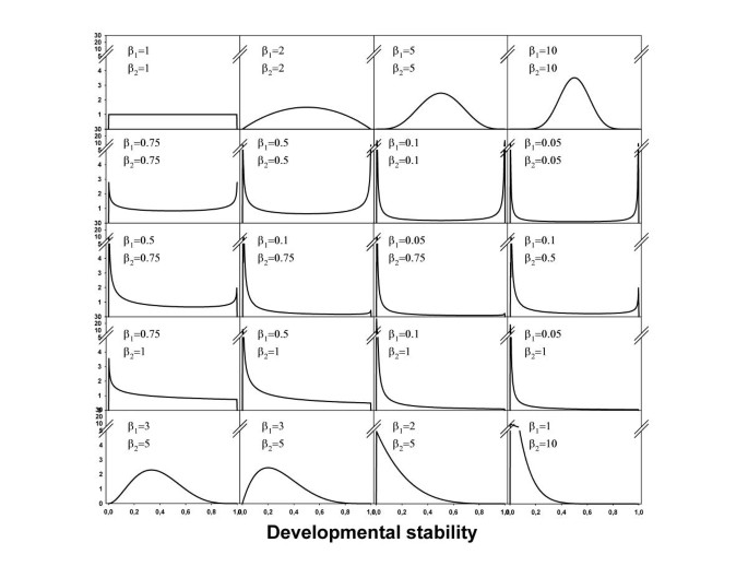
Overview of distributions of DS that were used to simulate datasets The bottom three rows of distributions are skewed to the left. The same right-skewed distributions (obtained by interchanging β1 and β2) are also used (Table 1)
Results
The beta-distributions applied to model variation in DS generated a broad range of CV values for both DS and DI and of values of R (Table 1). In agreement with earlier results [13, 15], R was closely and positively associated with the CV of DI (Fig. 2). Values larger than 100% were required to obtain relative large values of R (>0.4). However, when examining the relationship at the level of DS, the association was negative (Fig. 2) indicating that only small amounts of variation in DS were required to obtain large values of R. For example, the largest value of R was obtained with a left skewed distribution of DS with a values of CV equal to only 17% (Table 1), hereby lying well within the range of morphological and fitness traits [13].
Figure 2
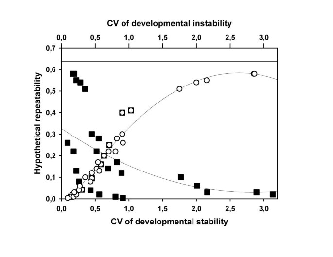
Relationship between the coefficient of variation (CV) of both DS and instability and the hypothetical repeatability (R) Mean values and their standard deviation were obtained for a range of distributions of variation in DS. Details are provided in Figure 1 and Table 1. The theoretical upper limit of R equals 0.637 and is indicated by a horizontal line
Table 1 Results of numerical simulations Hypothetical repeatability of single trait unsigned asymmetry (R) and the coefficient of variation of DS (CV-DS) and instability (CV-DI) for simulated datasets were the distribution of DS followed a beta-distribution with different shapes (Fig.1). Results are means (SD) of 1000 samples of 10000 observations.
When examining Table 1 and Figure 2 in more detail, the overall negative association between R and the CV of DS did not appear to hold when the distribution of DS was symmetrical. Values of the CV's of DS and DI were identical and in both cases correlated positively with R. Thus, the association between the CV's of DS and R depends on the shape of the distribution of between-individual variation in DS.
Empirical estimates of the distribution of DS: a Bayesian model
In addition to the amount of variation, distributional characteristics of DS have an important impact on the relationship with values of R. As a result, values of R do not consistently reflect variation in DS and distributional characteristics of variation in DS need to be evaluated additionally. Below we first propose a statistical model based on Bayesian statistical principles, to estimate the distribution of DS and then apply it to both simulated and empirical data.
A Bayesian approach
The first step in any Bayesian analysis is to construct the full joint probability model of both the parameters of the model (a vector indicated by θ) and the data (indicated by y) as p(θ,y). This model can be decomposed in a set of sub-models, which are then completed with prior distributions [p(θ)]. In contrast to more traditional methods, parameters are considered to be stochastic rather than fixed. Conclusions about the parameter space θ are made in terms of probability statements conditional on the data y. These probability statements are based on the posterior distribution of each parameter [p(θ|y) = p(θ)p(y|θ)/p(y)] which can either be obtained analytically or by Monte Carlo Markov Chain simulation (MCMC) [19, 20].
Bayesian statistics were introduced into the field of DS and FA to model heterogeneity in measurement error (ME) [5] and to obtain unbiased estimates of DI-fitness associations [17]. One aspect of these models – which we adopt here – was to construct a fully Bayesian mixed-effect regression model. Each observation (i.e. measurement on each side) is modelled as a sample from a normal distribution with mean equal to the unknown trait value and variance equal to the degree of measurement error (σ2 ME):

where i = 1..N and j = 1..K with N = number of individuals and K = number of within subject repeats.
The expected value of a single measurement (i.e. expected [i,j]) is modelled by the sum of a population-specific part (i.e. the fixed-effects) and an individual-specific part (i.e. the random-effects). As fixed-effects an intercept and a slope are included, modelling directional asymmetry. An individual-specific random intercept (interc_ind [i]) and slope (slope_ind [i]) model individual variation in size and asymmetry around this regression line, reflected in ind_profile [i,j]. Random effects are assumed to follow a normal distribution with zero means and variances reflecting variation in size (σ2 size) and asymmetry (σ2 FA) respectively:
The model is then completed with the following prior distributions [19]:

The parameter estimates obtained from this model have exactly the same interpretation as for the empirical Bayes' approach [21]. However, because each parameter is treated as a stochastic variable, standard deviations become slightly larger [5]. The main importance of this part of the model is to obtain unbiased estimates of individual asymmetry, here treated as distributions instead of fixed values.
The next step in the model – and this part of the model differs from the previous two approaches – is to establish a link between the observable individual asymmetry and both the unobservable DN and DS. This can be achieved by assuming that each individual asymmetry value reflects a sample from a normal distribution with zero mean and variance σ2 FA [i], the latter representing the individual-specific degree of DI [10]. Note that in contrast to equation 8, here each individual is assumed to have a specific degree of DI, or in other words that there is variation in the underlying DI. In agreement with equation 3, DI can be modelled as the joint effect of DN and DS, where DS follows a beta distribution:
The so-called hyperparameters β1 and β2 and DN are given the following prior distribution with a lower limit of zero (i.e. parameters of beta distribution or variances cannot be negative):
N(10,1000) (12)
Posterior distributions of the parameters of interest could in theory be obtained analytically, but in practice our model is to complex. Alternatively, simulation techniques provide a convenient option. The computer package WINBUGS applied here to analyse the different datasets, makes use of MCMC with Gibbs sampling and the Metropolis-Hastings algorithm [19, 20]. In each analysis performed below, 5 independent chains were run with a burn in period of 500 iterations and 1000 iterations from which the posterior distributions were estimated. Each distribution is thus based on 5000 iterations. Convergence was checked with the Gelman and Rubin 'shrink factor' in combination with visual inspection of the chains and their degree of autocorrelation [22, 23]. Unless mentioned otherwise, convergence behaviour was good.
The analysis of simulated data
In order to evaluate the usefulness and limitations of the proposed technique, datasets with six different distributional characteristics of DS and three different sample sizes were generated and subsequently analysed. Posterior means and medians of DN are given in Table 2. These estimates appeared to be biased upward for the two left-skewed (β1>β2) distributions and the bimodal one. For the other shapes of the distribution of DS (see Fig. 3), estimates of DN were more accurate. This result is not unexpected. In left-skewed distributions relatively few individuals are developmentally unstable (i.e. low DS), while those individuals contain most information about the size of DN.
Figure 3
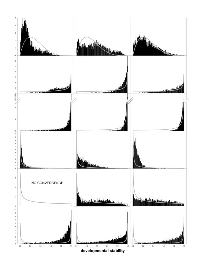
Posterior distributions of DS Posterior distributions indicated by the black bars were obtained for datasets with three different sample sizes (left: N = 500; middle: N = 1000; right: N = 5000) and six different underlying shapes generated from different beta-distributions (row 1: β1 = 2, β2 = 5; row 2: β1 = 1, β2 = 0.5; row 3: β1 = 1, β2 = 0.1; row 4: β1 = 0.1, β2 = 1; row 5: β1 = 0.5, β2 = 1; row 6: β1 = 0.1, β2 = 0.1; indicated by the gray lines)
Table 2 Posterior mean (SD) and median values of the degree of developmental noise (DN). Data were generated for three different sample sizes and for six different shapes of the distribution of DS, as determined by two parameters β1 and β2 of the beta-distribution. The true underlying value of DN equalled 1. Estimated distributions of variation in DS are presented graphically in Figure 3.
Figure 3 shows expected and estimated distributions of between individual variation in DS. In most occasions the estimated distribution, although sometimes roughly, approximated the expected distribution (Fig. 3), except for the bimodal case where the peak of developmentally unstable individuals was not detected (Fig. 3 bottom row). In general, and ignoring the bimodal case, the shape of the distribution was detected even so for sample sizes of 500 individuals. Still, in one occasion the MCMC failed to converge. Convergence problems occur even more frequently for smaller sample sizes (i.e. N = 250), but upon convergence the obtained estimate of the distribution reflected the true shape (data not shown).
An example where the method fails
We treat DI as the joint effect of DN and DS (equation 3). Because the observable FA of a trait depends on the magnitude of DI, DN and DS can only be separated statistically from each other under particular conditions. That is when one of the two is held constant (in our simulations we keep DN constant) and when values of the other span the whole range of possible values (between 0 and 1 for DS). Suppose we limit the distribution of between-individual variation in DS between 0 and 0.5 and use a value of DN equal to 1. The variance component DI that leads to the observable FA values, then varies between 1 and 0.5. However, the same range can be obtained for, for example, a value of DN equal to 10 and DS ranging between 0.1 and 0.05. In other words, different solutions are equally likely. This is illustrated by the posterior distributions of DS and DN obtained for this particular example with a sample of 500 individuals (Fig. 4). For both DS and DN multimodal distributions are obtained and the MCMC's did not show convergence. Together with problems of small sample sizes a restricted range of the distribution of DS appears to lead to convergence problems.
Figure 4
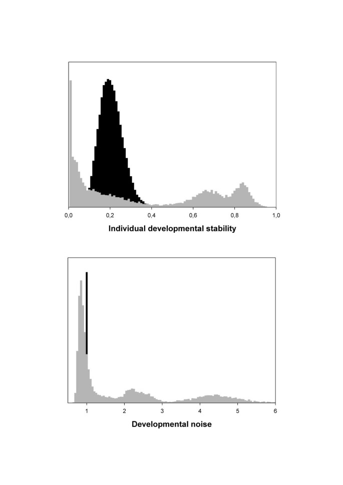
Expected (black) and observed (gray) distribution of between-individual variation in DS (top graph) and population level developmental noise (bottom graph)
Patterns in the real world
Analyses of simulated data showed that the presented method provides reliable estimates of the distribution of DS under a variety of conditions. In addition, unless the MCMC failed to converge, the obtained distributions approximated the underlying ones. We therefore assume that convergence offers a good criterion for the reliability of obtained results. We apply the above model to 8 datasets from 5 different species and 7 different traits (Table 3), following the specifications detailed above. In two cases, the MCMC did not converge. The hypothetical repeatabilities in these cases were low (Table 3) and not significantly different from zero. Thus, the available data do not allow concluding that variation in individual DS was present. Distributions of between-individual variation in DS of the remaining six samples – which did show good convergence behaviour – are given in Figure 5. Distributions are remarkably similar in shape, all showing a highly left skewed distribution, irrespective of the value of the hypothetical repeatability. In addition, values of R were not correlated with the degree of variation in DS (Fig. 6).
Figure 5

Between-individual variation in DS as estimated for six empirical datasets
Figure 6
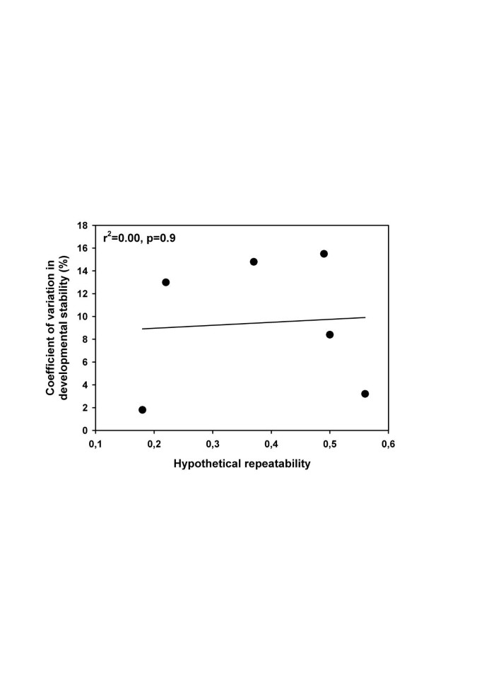
Association between the hypothetical repeatability and the coefficient of variation in DS for six empirical datasets
Table 3 Overview of empirical datasets used to estimate developmental noise and the distribution of variation in DS simultaneously.