A novel method for sparse channel estimation using super-resolution dictionary (original) (raw)
1 Introduction
Traditional channel estimation methods on orthogonal frequency division multiplexing (OFDM) systems commonly assume that the channel has rich multipath and require a large number of pilots to obtain more accurate state information of the channel, which seriously reduce the utilization efficiency of the channel. Meanwhile, traditional methods of linear channel estimation already attained optimal estimation performance such as utilization efficiency, so it is difficult to improve them further. To overcome the bottleneck, we need to explore the own characteristic of the channel. More and more experimental evidences show that the sparse distribution of reflectors in space makes the transmission channel sparse.
The research on sparse wireless channel has already begun since the 1990s. Cotter and Rao utilize matching pursuit (MP) algorithm to estimate a small amount of non-zero channel taps in a single-carrier selective channel [1]. MP algorithm on decision feedback equalizer can effectively improve the performance of channel estimation. Compared with MP algorithm, the method proposed by Raghavendra and Giridhar estimates the tap position in a frequency-selective channel based on generalized Akaike information criterion and least squares (LS) algorithm, which greatly reduces the calculation burden of LS algorithm [2]. However, the above results were basically obtained by simulation and lacked relating theory analysis. In recent years, Donoho and Candes et al. propose a novel theory, i.e., compressed sensing, on the basis of functional analysis and approximation theory. The theory suggests that if the signal is sparse in a certain domain, it can be accurately reconstructed by a small amount sampling signal with high probability [3, 4]. Bajwa et al. firstly applied compressed sensing (CS) theory for channel estimation and proposed the concept of compressive channel estimation (CCE) [5]. In the literature [5, 6], Bajwa made a feasibility analysis of CCE and extended it to a doubly selective channel. The literature [7] gives a virtual channel model by Nyquist sampling for physical transmission environment in the angle-delay-Doppler domain and makes a comparison between CCE and LS. Meanwhile, aiming at acoustic OFDM systems, Berger et al. proved that CS channel estimation is superior over the traditional linear channel estimation method, which is reflected in the experimental data, like root-MUSIC and ESPRIT algorithms [8, 9]. Taubock and Hlawatsch transform a doubly selective channel model to a solvable basis pursuit inequality constraint model, utilize the pilot signal as the key measurement that CS reconstruction requires, and analyze the sparsity of the channel parameter in the delay-Doppler domain [10]. However, it was concluded from the analysis that the energy leakage problem caused by discrete truncation of time domain and limited bandwidth obviously deteriorates the channel’s sparsity which limits the performance improvement of CS-based channel estimation methods. To solve the problem, Taubock et al. propose an iterative basis optimization procedure that aims to maximize sparsity [11, 12]. Although the method proposed by Taubock achieves significant performance gains, its basis optimization, which adds additional complexity, has to be performed before data transmission. Aimed at common problems caused by time delay and Dopler frequency shift of non-integer multiple samples, we use a super-resolution over-complete dictionary to improve the performance of channel estimation. The dictionary only increases the run time of the sparse reconstruction procedure with the increase of basis. We find that the over-complete dictionary representation of the channel is much sparser than the classical delay-Doppler representation in most cases, and it can effectively reduce the usage of pilots and improve the estimation performance.
The rest of this paper is organized as follows. Section 1 introduces CS theory and Section 2 introduces the OFDM system model. Section 3 analyzes the energy leakage of the channel in the delay-Doppler domain firstly, then uses the super-resolution dictionary instead of Fourier basis to enhance the sparsity of the channel, and next presents the CS-based channel estimation method. In Section 4, we present numerical results. Finally, Section 5 concludes the paper.
2 Compressed sensing theory
CS is a novel and highly promising theory that combines applied mathematics and signal processing. It breaks through the limitation of traditional Nyquist sampling and greatly reduces sampling frequency, data storage, and transmission burden. In CS, if a vector x∈ ℝ N is _K_-sparsity, or approximate K_-sparsity, it can be represented by using K(≤_N) non-zero coefficients [3]. Then, a linear measurement value about x can be obtained by selecting appropriate measurement matrix Φ∈ ℂ M × N (M<N), as shown in (1). Only M measurements within y can be utilized to reconstruct the original signal with very high probability.
The dimension number of y is far less than that of x, so equation array (1) is underdetermined. However, in view of x which is _K_-sparse, it is only required to obtain K non-zero coefficients and their position. Candes et al. have proved that if the number of measurement _M_=O(K log(N)), and the measurement matrix satisfies the constraint of restricted isometry property (RIP), signal x can be reconstructed by solving the _l_0-norm minimization in (2) [3].
min x x 0 subject toy=Φx
(2)
Tao et al. already proved that Gaussian random measurement matrix, random partly Fourier measurement matrix, and Toeplize random matrix can satisfy the RIP criterion with very high probability [4], i.e., any N dimension _K_-sparsity vectors a all satisfy the following rule:
1 − δ k a 2 2 ≤ Φa 2 2 ≤ 1 + δ k a 2 2
(3)
where δ k ∈(0,1) is a constant.
Unfortunately, _l_0-norm is not convex. Actually, this problem is NP hard and therefore cannot be solved in a reasonable amount of time. By now, there are many different algorithms to solve it. Orthogonal matching pursuit (OMP) becomes a popular way in CS theory because it is simple for computation and easy for implementation [13]. OMP algorithm transforms the problem, _l_0-norm minimization, to a relative simple problem shown in (4):
x= min x ′ ∈ ℝ N x ′ 0 subject to Φ x ′ − y 2 ≤ε
(4)
where ε is the upper bound of the noise level. The basic idea of OMP algorithm is how to select the column vector of measurement matrix Φ by utilizing the greedy iteration way and reconstruct the signal by computing the support vector set on iterative algorithm of parameter x[13].
3 OFDM system model
3.1 System model
We describe a generalized cyclic prefix (CP) OFDM system shown in Figure 1. The discrete-time transmission can be written as
x n = 1 K ∑ l = 0 L − 1 ∑ k = 0 K − 1 x l , k e j 2 πkn / K g n − lN
(5)
Figure 1
OFDM system model. The baseband-equivalent doubly selective channel h(t,τ) includes physical channel _h_ch(t,τ), transmitter filter _f_tr(t), and received filter _f_rec(t).
where K is the number of subcarriers, L is the number of transmitted symbol periods, and N denotes the symbol duration. _N_CP=N_−_K is the guard interval for the CP which is used to avoid the intersymbol interference (ISI). x l,k denotes the l th symbol transmitted at subcarrier k, and discrete transmit pulse _g_[_n_] is 1 on [0,_N_] and 0 otherwise.
The baseband-equivalent doubly selective channel h(t,τ) includes physical channel _h_ch(t,τ), transmitter filter _f_tr(t), and received filter _f_rec(t), so we have
h t , τ =∫∫ f rec s f tr τ − s − θ h ch t − s , θ dsdθ
(6)
In the receiver, the received signal after being sampled with period T s is given by
r n = ∑ θ ∈ ℝ h n , θ x n − θ +z n
(7)
where _h_[n,_θ_]=h(n T s ,θ T s ) and _z_[_n_]=z(n T s ) is discrete-time noise.
Assuming that the receiver is synchronous, if signal _r_[_n_] is demodulated, we can obtain
r l , k = 1 K ∑ n = − ∞ ∞ r n e − j 2 πk n − lN / K γ n − lN
(8)
where _l_=0,1,…,_L_−1, _k_=0,1,…,_K_−1, and _γ_[_n_] is only 1 in [N_−_K,_N_−1] and 0 otherwise. Combining (5), (7), and (8), we have
r l.k = H l , k x l , k + z l , k
(9)
where z l , k = 1 K ∑ n = − ∞ ∞ z n e − j 2 πk n − lN / K γ n − lN denotes the noise or the interference terms. H l,k is the system channel coefficients which will be analyzed in the following sections.
3.2 Doubly selective fading channel
According to the wide-sense stationary uncorrelated scattering (WSSUS) model, the time-varying multipath channel is expressed as [14]
h ch t , τ = ∑ q = 1 P η q δ τ − τ q e j 2 π v q t
(10)
where P is the number of multipath components and η q , τ q , and v q are the attenuation coefficient, the delay, and the Doppler shift of path q th, respectively. δ denotes the Dirac delta function. We obtain the delay-Doppler spreading function S(v,τ) via Fourier transform.
S v , τ = ∫ h t , τ e − j 2 πvt dt = ∑ q = 1 P η q δ τ − τ q δ v − v q
(11)
Assuming that physical channel h(t,τ) does not vary in the area of received filter _f_rec(t), Equation 12 can be derived from Equation 6.
h ( t , τ ) = ∬ f rec s f tr τ − s − θ h ch t , θ dsdθ = ∫ ψ τ − θ h ch t , θ dθ = ∑ q = 1 P η q ψ τ − τ q e j 2 π v q t
(12)
where ψ(τ_−_θ)=_f_tr(t)⊗_f_rec(t). After discretizing Equation 12, we have
h n , θ = ∑ q = 1 P η q ψ θ T s − τ q e j 2 π v q n T s
(13)
Due to the non-linear relation between _h_[n,_θ_] and channel parameters [η q ,v q ,τ q ], it is difficult to analyze the channel by utilizing Equation 13. It caused us to search for a new model with less parameters.
4 Sparse channel estimation using a dictionary
4.1 The effect of sparsity caused by energy leakage
Because the basis expansion model (BEM) [15] is simple for calculation and independent on statistical characteristics of the channel, it is widely used in time-varying multipath channel estimation. To compute r l,k in (8) for all _l_=0,1,…_L_−1, the discrete-time received signal _r_[_n_] has to be known for _n_=0,…,_N_0−1, where _N_0=L N. The discrete time channel impulse response _h_[n,_θ_] in Equation 13 can be represented by BEM with a period of _N_0[16], so we have
h n , θ = ∑ i = − J J S h i , θ e j 2 πin / N 0
(14)
where J satisfies J/(N_0_T s )≥_v_max/2 and _v_max/2 denotes the single-sided maximum Doppler shift. S h [i,_θ_] is the discrete delay-Doppler spread function:
S h i , θ = 1 N 0 ∑ n = 0 N 0 − 1 h n , θ e − j 2 πin N 0 = ∑ q = 1 P η ′ q ψ θ T s − τ q dir N 0 i − v q T s N 0
(15)
where dir N (x)= sin (π x)/(N sin(π x/N)), η q ′ = η q e jπ v q T s − i / N 0 N 0 − 1 , and _θ_=0,…,D_−1. D_≥_τ_max/T s denotes the number of discrete time-delay sampling points. It is obvious that if the maximum time-delay satisfies τ_max≤_N_CP, the intersymbol interference can be eliminated. And if the ideal filter f tr t = f rec t = 1 / T s sinc t / T s is applied, where sin_c(x)=sin(π x)/(π x), ψ(θ T s −_τ q )≈ sin_c(θ_−_τ q /T s ) can be obtained and applied in Equation 15. So we have
S h i , θ = ∑ q = 1 P η ′ q Λ q i , θ
(16)
where
Λ q i , θ =sinc θ − τ q T s dir N 0 i − v q T s N 0
(17)
Combining (7), (9), and (14), we can derive the channel coefficient H l,k
H l , k = ∑ θ = 0 D − 1 ∑ i = − J J − 1 S h i , θ e − j 2 π kθ K − il L A γ , g θ , i N 0
(18)
where A γ , g θ , i / N 0 = ∑ n γ n g n − θ e j 2 πin / N 0 is the cross-ambiguity function. Therefore, we can analyze the sparsity of Λ q [i,_θ_] instead of S h [i,θ_]. From Equation 11, the delay-Doppler function S(v,τ) consisted of the Dirac function in delay-Doppler point (τ q ,v q ) which corresponds to reflecting path q and is supposed to be sparse. However, the Dirac function is replaced by sin_c(x) and dir N (x) in S h [i,_θ_]. Only when τ q /T s and v q T s _N_0 are all integers, Λ q [i,θ_] can be simplified to the Dirac function. The reason is that sin_c(x) and dir N (x) are equal to 1 on _x_=0 and 0 otherwise, as shown in Figure 2. Under any other conditions, Λ q [i,_θ_] is not equal to 0 for any i and θ. In other words, the peak energy of the discrete delay-Doppler function may have leakage to the near delay-Doppler area. Figure 3 demonstrates the leakage effect of S h [i,_θ_] where _P_=10, _N_CP=16, _K_=25, and _L_=16. η q , τ q /T s , and v q T s _N_0 are random variables.
Figure 2
Functions sin c ( x ) and dir N ( x ). sin_c_(x) and dir N (x) are equal to 1 on _x_=0 and 0 otherwise, but their intensity decreases due to the decay.
Figure 3
Modulus of the expansion coefficients for DFT basis. Since the fading of sin_c_(x) and dir N (x) is slow, a lot of coefficients should not be neglected which decrease the sparsity of the channel. The parameters are _P_=10, _N_CP=16, _K_=256, and _L_=16. η q , τ/T s , and v q T s _N_0 are random variables.
From Figure 3, the peak energy of S h [i,_θ_] leaks to the near delay-Doppler area, and then its value would fade and approximate to 0 gradually. Therefore, S h [i,θ_] is approximate sparse, i.e., the channel coefficient H l,k is approximate sparse in the delay-Doppler domain. However, the fading of sin_c(x) and dir N (x) is slow, and a lot of values in S h [i,_θ_] cannot be neglected. It seriously influences the sparsity of the channel and the estimation performance of the channel.
4.2 Sparsity enhancement using the super-resolution dictionary
In real wireless channels, the time delay and Doppler frequency shift of non-integer times sampling points exist generally. They seriously influence the sparsity of channel coefficient H l,k in the time delay and Doppler domain and do not satisfy the prerequisite condition. Hence, how to avoid the energy leakage is a very important issue in channel estimation. Essentially, the channel energy leakage is actually introduced by channel discrete characterization, and the sparsity of the channel itself does not disappear. Therefore, if we can improve the accuracy of channel discrete characterization, it would greatly reduce the energy leakage. Therefore, improving the discrete accuracy of the channel impulse response reduces the energy leakage [17].
Assuming that _h_[n,_θ_] can be represented by BEM with a period of λ _N_0, we have
h n , θ = ∑ i = − J J S λ i , θ e j 2 πin / λ N 0
(19)
where J/(λ N_0_T s )≥_v_max/2.
Let h θ λ = h 0 , θ , … , h λ N 0 − 1 , θ T and S θ λ = S λ − J , θ , … , S λ J − 1 , θ , we can derive S θ λ based on LS and obtain
min S θ λ h θ λ − 1 λ N 0 F λ S θ λ 2
(20)
where F λ = 1 ⋯ 1 e − j 2 πJ λ N 0 ⋯ e j 2 π J − 1 λ N 0 ⋮ ⋯ ⋮ e − j 2 πJ λ N 0 − 1 λ N 0 ⋯ e j 2 π J − 1 λ N 0 − 1 λ N 0 .
Then,
S θ λ = F λ ‡ h θ λ = 1 λ N 0 F λ H h θ λ
(21)
where S θ λ corresponds to 2_J_+1 Doppler sample point under λ times over-sampling.
We may define S θ , m λ = S λ − a m λ + m , θ , … , S λ b m λ + m , θ and h θ =[_h_[0,_θ_],…,_h_[_N_0−1,_θ_]]T, where a m =(J+m) mod λ and b m =(J_−_m) mod λ. It is easy to prove Equation 22:
S θ , m λ = min S θ , m λ D m λ h θ − 1 N 0 F m λ S θ , m λ 2
(22)
where D m λ =diag 1 , e − j 2 πm λ N 0 , … , e − j 2 πm N 0 − 1 λ N 0 T and
F m λ = 1 ⋯ 1 e − j 2 π a m / N 0 ⋯ e j 2 π b m / N 0 ⋮ ⋯ ⋮ e − j 2 π a m N 0 − 1 / N 0 ⋯ e j 2 π b m N 0 − 1 / N 0
.
Then,
S θ , m λ = F m λ ‡ D m λ h θ λ = 1 N 0 F m λ H D m λ h θ
(23)
Equation 23 corresponds to taking the (a m +b m +1) samples around zero from the critically sampled Doppler spectrum of the m/(λ N) frequency-shifted version of h θ . So all samples (_m_=0,1,…,λ_−1) can deduce 2_J+1 Doppler frequency shift point. By replacing D m λ , F m λ , and h θ into Equation 23, we have
S λ i , θ = ∑ q = 1 P η q ψ θ T s − τ q e jπ v q T s − i λ N 0 N 0 − 1 × dir N 0 π i − λ v q T s N 0
(24)
From Equations 24 and 16, we find that dir N 0 π i − v q T s N 0 in Equation 16 is replaced into dir N 0 π i − λ v q T s N 0 . So if v q T s _N_0=n/λ, dir N 0 π i − λ v q T s N 0 can be transformed into a Dirac function. The higher the parameter λ is, the more the sample of the Doppler spectrum is. And when the position of the sample is closer to the real position, the problem of energy leakage would greatly be reduced. Admittedly, a part of the Doppler spectrum still results in a certain energy leakage; however, its value is very small. Letting I denote all integer set which satisfied |i_−_λ v q T s N_0|≤_Δ i in the area of i_∈{−_J,…,J}, the energy sum of samples in which the distance v q T s _N_0 in dir N 0 π i − λ v q T s N 0 is larger than Δ _i_∈{2,3,…} can be given.
∑ i ∉ I dir N 0 π i − λ v q T s N 0 2 = ∑ i ∈ I sin π i − λ v q T s N 0 N 0 sin π i − λ v q T s N 0 / N 0 2 ≤ ∑ i ∈ I 1 N 0 sin π i − λ v q T s N 0 / N 0 2 ≤ 2 N 0 2 ∫ Δi − 1 ∞ dx sin 2 πx / N 0 = 2 N 0 π cot π N 0 Δi − 1 ≤ 1 π Δi − 1
(25)
Figure 4 shows the leakage effect of dir N 0 π i − v q T s N 0 and dir N 0 π i − λ v q T s N 0 , where v q T s _N_0=0.4 and v q T s _N_0=0.5.
Figure 4
Comparison between dir N 0 π i − λ v q T s N 0 and dir N 0 i − v q T s N 0 . dir N 0 π i − λ v q T s N 0 has a quicker fade speed of side lobe and a smaller value of side lobe than dir N 0 i − v q T s N 0 . (a) v q T s _N_0=0.4, _λ_=2. (b) v q T s _N_0=0.5, _λ_=2.
Similarly, we can apply the same method to solve the energy leakage problem in the time-delay domain [18]**,**[19]. Lastly, equivalent discrete-time baseband channel frequency response is given by
H l , k = ∑ θ = 0 D − 1 ∑ i = − J J − 1 S D i , θ e − j 2 πkθ / λ delay K e j 2 πil / λ Doppler L × A γ , g θ , i / N 0
(26)
where D T s /_λ_delay≥_τ_max, _λ_delayand _λ_Dopplerare the over multiple number of delay and Doppler, respectively, and A γ,g(θ,i/_N_0) is the same as that in Equation 17.
Redundant dictionary U is defined by U kL + l , i + J D + θ = e − j 2 π kθ / λK − ni / λ N 0 , h kL + l = H l , k , and g i + J D + θ = S D i , θ A γ , g ′ θ , i / N 0 . Obviously, g is sparse according to the above analysis. So we can obtain the vector form of Equation 26:
Especially, if _λ_=1, U is the 2-D Fourier basis as used in Equation 18. Under the same conditions as those in Figure 3, Figure 5 shows the distribution of coefficient g in the dictionary domain.
Figure 5
Sparsity enhancement obtained with the over-complete dictionary corresponding to λ =2. The effective value is much less than that in Figure 3; the parameters are the same as those in Figure 3 except the basis.
Obviously, the effective value g in Figure 5 is less than that in Figure 3. So the channel coefficient corresponding to _λ_=2 has a higher sparsity. To analyze the sparsity in the dictionary domain better, we utilize OMP algorithm to solve _S_-sparse approximation and obtain the most S maximum value in g. From Figure 6, with the increase of S, the mean square errorE[|h− h ̂ S | 2 ]would decrease gradually and would be close to 10−1, i.e., we can obtain 90% channel energy based on S strongest atoms. If λ is higher, the atoms that satisfy the required mean error are fewer. So we can conclude that if λ is higher, the sparsity of frequency response h is higher in the over-complete dictionary.
Figure 6
MSE of sparse approximation of h in Equation 27.We utilize OMP algorithm to solve _S_-sparse approximation and obtain the most S maximum value in g; a redundant basis leads to significantly fewer terms than Fourier basis.
4.3 The estimation of the sparse channel based on the dictionary domain
Assuming that l , k ∈P, wherePis the pilot set, the total number of pilot point isQ= P . The number of pilots must satisfy the lowest demand of compressive sensing theory to represent the measurement signal without distortion. The literature [14] gives the limitation of the number of measurement samples required by OMP. N m ≥K S ln(N r /δ), where S denotes sparsity. Commonly, _K_≤20 is reasonable. If S is too large, we may also set _K_≈4 and δ_∈(0,0.36). OMP may reconstruct a signal with 1−2_δ probability. So we can select the suitable number of pilots, Q_≥_N m .
According to (9), the estimation of the channel coefficient in the pilot is given by
H ~ l , k = r l , k x l , k = H l , k + z l , k
(28)
Let h Δ =h l , k ∈ P , U Δ =U l , k ∈ P be the matrix corresponding to the pilot point, and z Δ be the set of z ~ l , k in l , k ∈P. We have
According to the above analysis, we can conclude that g is sparse. So Equation 27 is a standard equation of CS. Measurement matrix U Δ is a structured random matrix which is formed by selecting a row vector of unitary matrix corresponding to the pilot point. If we select the position of the pilot uniformly and randomly and Q is large enough, the normalized matrix 1 / Q U Δ has a small constraint isometric constant with very high probability. In other words, we can obtain very good reconstruction performance. So we can obtain Equation 30 from Equation 29.
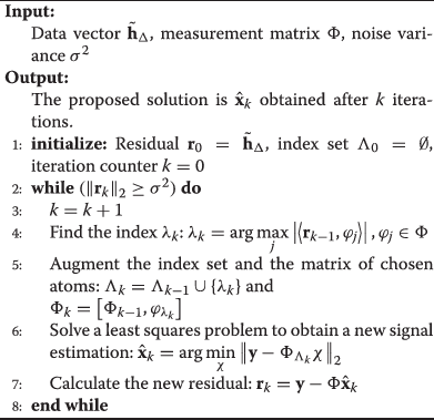
whereΦ= KL / Q U Δ andx= Q / KL g. Therefore, we may realize channel equalization based on CS theory. The following are the detailed steps:
- Obtain the estimation H ~ l , k of the channel coefficient according to Equation 28, and then combine all H ~ l , k to form h ~ Δ .
- Utilize OMP to obtain an estimation x ~ of x based on known h ~ Δ and Φ according to Equation 30. The detail of realization refers to Algorithm 1. After rescaling x ~ , we can obtain estimation value g ~ , as well the spread coefficient S D [i,_θ_] corresponding to the dictionary.
- Compute all channel coefficient h ~ by utilizing Equation 27 based on known g ~ and U.
The run time of OMP mainly depends on the index set Λ k selected in the iteration process. We need to select the optimal atom O(D(2_J_+1)) from D_×(2_J+1) atom. So with the increase of λ, the number of time-delay sample D and the number of Doppler sample J would increase exponentially. However, with the increase of λ, the channel sparsity would be enhanced and the iteration times required by OMP would reduce. Lastly, it can save a certain run time.
Algorithm 1 Steps of reconstitution
5 Simulation and analysis
In this section, we present numerical results to analyze the performance of the CS-based channel estimation algorithm using the over-complete dictionary. The following are the relating simulation parameters: carrier frequency f c =2 GHz, bandwidth _B_=10.24 MHz, sub-carrier number _K_=1,024, the length of cyclic prefix N CP =128, and sample period T s =0.1 ms. We may utilize the channel simulation tool IlmProp [20] based on the geometrical structure of space to simulate a doubly selective fading channel. The simulated frame for the OFDM block has eight symbols, i.e., _L_=8. In the simulated environment, the distance between the transmitter and the receiver is 2,000 m, and 10 reflectors, in which 2 reflectors are distributed within 150 m from the transmitter, form 10 multipath clusters, which satisfy the Gaussian distribution. The random speed of each path is less than 100 m/s and the acceleration is less than 20 m/s2. Assume that the noise _z_[_n_] is additive white Gaussian noise (AWGN), in which the mean is 0 and the variance is σ2. So the signal-noise ratio (SNR) of the symbol block is given by
SNR= ∑ n = 0 N 0 − 1 E r n − z n 2 ∑ n = 0 N 0 − 1 E z n 2
(31)
In addition, simulation tools are MATLAB 2009 and an Intel Core PC with a 2.8-G processor and 1.5-G RAM.
To begin with, we give the performance comparison for a variety of algorithms under different SNR conditions. The SNR varies within −10∼20 dB. For LS channel estimation, we used two different rectangular pilot constellations, i.e., selected uniformly 6.5% and 12.5% of all symbols for pilots, respectively. For CS-based estimation, we select randomly 6.25% of all symbols for pilots and three different basis, i.e., Fourier basis (DFT) (i.e., _λ_=1) [10], iterative optimize basis [12], and over-complete dictionary (DIC) (_λ_delay=_λ_Doppler=2,_λ_delay=_λ_Doppler=4). Figure 7 gives the MSE comparison of different algorithms under SNR. Figure 8 shows the bit error ratio (BER) comparison of equalization decoding. Both figures suggest that when we only apply 6.25% resource as pilots, the performance of LS estimation is much bad; the reason is that the distribution of the pilot cannot satisfy the Nyquist sampling criterion. However, when OMP algorithm also applies 6.25% resource for the pilot, the performance of the channel estimation proposed in this paper is better than that of LS estimation that applies 12.5% resource for the pilot. So the utilization efficiency of the spectrum is improved obviously. In addition, OMP algorithm on the over-complete dictionary domain has a better performance than the traditional algorithm on the delay-Doppler domain. When _λ_=2, the performance on the over-complete dictionary domain approaches that on the iterative optimize basis. And when _λ_=4, the performance on the over-complete dictionary domain is better than that on the iterative optimize basis. With the increase of the λ, the BER performance of OMP algorithm using over-complete dictionary is close to that of ideal channel estimation. So the higher is λ, the better is the reconstruction performance of OMP and the higher is the estimation accuracy.
Figure 7
MSE performance in different SNR environments. The compressed sensing methods can increase their performance significantly by using dictionaries with a finer resolution (for OMP, _λ_=2,4); OMP_DFT, OMP_OPT, and OMP_DIC represent Fourier basis, iterative optimize basis, and dictionary used in OMP algorithm, respectively.
Figure 8
BER performance in different SNR environments. With the increase of λ, the bit error rate is gradually reduced and reaches the ideal channel estimation.
Although the performance of the dictionary on _λ_=4 is the best, its complexity is also the highest, as shown in Table 1. Considering the reconstruction time only, iterative optimize basis is the optimal except for LS estimation. However, the method based on iterative optimize basis needs extra 163.8541 s to compute the optimal basis. But, in the channel estimation algorithm proposed in this paper, we can produce the dictionary by FFT. The method only enlarges the size of the reconstructed atomic set and does not need extra computation. By comparing the required time between _λ_=4 and _λ_=2, it can be concluded that the sparsity of the channel coefficient in the dictionary domain would be sparer with the increase of parameter λ. Meanwhile, the sparsity of the channel coefficient can also be influenced by the physical path and lower than the number of reflectors. Therefore, when _λ_=2, the channel estimation method based on the super-resolution dictionary domain has a certain advantage on the algorithm performance and computation complexity.
Table 1 The run time of different algorithms
Then, we present the performance comparison of different algorithms under the different numbers of pilot symbols. Here, SNR is assumed to be 0 dB, the number of pilot symbols varies within 3% ∼10%, and the other parameters are the same as those in the above simulation. Figure 9 shows that the performance is improved with the increase of the pilot number. Under the same accuracy condition, the higher the solution in the dictionary domain is, the less the required number of pilot is. For example, when MSN=−5 dB and _λ_=4, the required resource of pilots is only about 4%. If _λ_=2, the percentage is about 5%. However, the method based on Fourier basis needs about 7.5% resource. Figure 10 shows the comparison under the different numbers of pilots. With the increase of pilot number, BER would be close to the performance of ideal channel estimation. In other words, under the same performance of MSE or BER, the pilot number required by DIC is less than that by DFT and OPT. Hence, the sparse channel estimation based on the dictionary domain can effectively reduce the number of pilots and improve the spectrum efficiency.
Figure 9
MSE performance under the different numbers of pilot symbols. Dictionaries on _λ_=2,4 need less pilots than the optimized basis (OPT) and Fourier basis (DFT) in compressive channel estimation.
Figure 10
BER performance under the different numbers of pilot symbols. An increase in either the measure values or lambda can reduce BER.
Lastly, to reduce the computation complexity, we may apply different over-sampling times in the time-delay domain or the Doppler domain. In a wireless channel, we assumed that the random speed of each path cluster is less than 10 m/s and the acceleration is less than 1 m/s2, so the Doppler influence is not much serious. The other parameters are the same as those in the first simulation. Figures 11 and 12 show that when _λ_delay=4, _λ_Doppler=1, the performance of channel estimation is better than that of others. The accuracy performance on _λ_delay=_λ_Doppler=2 is almost the same as that on _λ_delay=2, _λ_Doppler=1; however, the former run time is about twice the latter, as shown in Table 2. Compared with that of the DFT and OPT, the run time of dictionary basis on _λ_delay=2, _λ_Doppler=1 is only slightly more than that of Fourier basis; however, the former performance is obviously better than the latter. Considering that the Doppler influence is not much serious, we only over-sample in the time-delay domain, so we can obtain an optimal selection in both computation complexity and performance. Similarly, we can also apply the same method in the Doppler domain.
Figure 11
MSE performance using different resolution dictionaries.When _λ_delay=4, _λ_Doppler=1, the performance of channel estimation is the best, while the accuracy performance on _λ_delay=_λ_Doppler=2 is almost the same as that on _λ_delay=2, _λ_Doppler=1; the over-sampling in the Doppler domain cannot improve the performance very much; the channel has a mild Doppler spread.
Figure 12
BER performance using different resolution dictionaries. The more sparse the channel is, the higher the degree of accuracy and the lower the BER we get.
Table 2 The required run time about different algorithms
6 Conclusions
This paper proposes a novel estimation method of a sparse and doubly selective channel based on CS theory. The method can reduce the problem of energy leakage caused by discrete truncation and the limited bandwidth by over-sampling in the delay-Doppler domain, enhance the sparsity of the equivalent channel in the dictionary domain, and then improve the performance of channel estimation. The results show that although the method based on the over-complete dictionary needs more computation, the estimation accuracy is improved obviously and the pilot resource is reduced very much. Lastly, compared with the increase of spectrum utilization, it is worth for more complexity.