Energy Deposition by Energetic Electrons in a Diffusive Collisional Transport Model (original) (raw)
0004-637X/862/2/158
Abstract
A considerable fraction of the energy in a solar flare is released as suprathermal electrons; such electrons play a major role in energy deposition in the ambient atmosphere, and hence the atmospheric response to flare heating. Historically, the transport of these particles has been approximated through a deterministic approach in which first-order secular energy loss to electrons in the ambient target is treated as the dominant effect, with second-order diffusive terms (in both energy and angle) being generally either treated as a small correction or neglected. However, it has recently been pointed out that while neglect of diffusion in energy may indeed be negligible, diffusion in angle is of the same order as deterministic scattering and hence must be included. Here we therefore investigate the effect of angular scattering on the energy deposition profile in the flaring atmosphere. A relatively simple compact expression for the spatial distribution of energy deposition into the ambient plasma is presented and compared with the corresponding deterministic result. For unidirectional injection there is a significant shift in heating from the lower corona to the upper corona; this shift is much smaller for isotropic injection. We also compare the heating profiles due to return current ohmic heating in the diffusional and deterministic models.
Export citation and abstractBibTeXRIS
Energy transport in solar flares involves a variety of mechanisms, such as nonthermal particle acceleration and propagation, thermal conduction, radiation, and bulk mass motions (see, e.g., Tandberg-Hanssen & Emslie 1988; Holman et al. 2011; Kontar et al. 2011a, for reviews). A significant fraction (e.g., Emslie et al. 2012) of the energy released is manifested as bremsstrahlung-emitting deka-keV electrons (see, e.g., Lin & Hudson 1976; Zharkova et al. 2011). These electrons propagate from the primary energy release site and deposit their energy in the ambient target principally through Coulomb collisions on ambient electrons (e.g., Brown 1972; Emslie 1978), with additional energy losses associated with ohmic dissipation of the neutralizing return current (e.g., Emslie 1980; Zharkova & Gordovskyy 2006) and with the turbulent environment through which they propagate (e.g., Bian et al. 2011; Kontar et al. 2011b).
Modeling of the Coulomb collision process has typically involved a test-particle approach involving systematic (secular) energy loss (e.g., Brown 1971, 1972; Emslie 1978), although numerical solutions of the Fokker–Planck equation, involving collisional diffusion in pitch angle (e.g., Leach & Petrosian 1981; Bespalov et al. 1991; MacKinnon & Craig 1991; Kontar et al. 2014) and energy (e.g., Jeffrey et al. 2014) in addition to the secular energy loss term have also been carried out. Bian et al. (2017) have shown that, while diffusion in energy can be justifiably neglected in a sufficiently cold target, diffusion of the accelerated electrons in angle is of the same order as secular change in angle and thus it is essential to include diffusive angular scattering processes in determining the spatial and angular distributions of the accelerated electrons in the target.
Knowledge of the energy deposition profile is a key element in determining the response of the solar atmosphere to flare heating (Mariska et al. 1989; Allred et al. 2015) and hence in interpreting the plethora of observations of Doppler-shifted and -broadened spectral lines (e.g., Antonucci et al. 1982; Emslie & Alexander 1987; Doschek 1990; Mariska et al. 1993; Bentley et al. 1994; Rilee & Doschek 2001; Landi et al. 2003; Brosius & Phillips 2004; Li et al. 2015a, 2015b, 2017; Milligan 2015; Reep et al. 2015; Tian et al. 2015; Brosius et al. 2016; Gömöry et al. 2016; Polito et al. 2016; Warren et al. 2016; Brosius & Inglis 2017; Kontar et al. 2017) in terms of the velocity differential emission measure (Newton et al. 1995) corresponding to candidate energy transport models. In this paper, we therefore build on the results of Bian et al. (2017) to derive a formula for the energy deposition profile associated with the passage of electrons through a cold target, where diffusion associated with angular scattering is explicitly taken into account. The results show that for unidirectional injection the spatial distribution of plasma heating differs noticeably from the simple deterministic treatment that has formed the basis for much of the modeling of both solar (Brown 1973; Mariska et al. 1989) and stellar (Allred et al. 2015) flares to date.
In Section 2, we present an analysis of collision-dominated electron propagation in a cold target, with angular diffusion taken into account; the results are presented as a solution for the electron flux F(E, z) (electrons cm−2 s−1 keV−1) at energy E and target depth z in terms of an integral over a Green’s function for electrons injected at a specified energy and pitch angle. In Section 3, we use this result to calculate the energy deposition rate as a function of z, both for unidirectional and isotropic injection cases. In Section 4, we briefly discuss the impact of diffusive angular scattering on the return current ohmic losses associated with driving the beam-neutralizing electron current though the finite resistivity of the ambient plasma. In Section 5, we discuss the results and present our conclusions.
Bian et al. (2017) have shown that the collisional transport of electrons in a cold target can effectively be modeled, in a first (local) approximation,3 by the one-dimensional transport equation (e.g., Kontar et al. 2014)
Here _f_0(v, z) (electrons cm−3 [cm s−1]−3) is the principal (isotropic) part of the electron phase-space distribution at speed v and distance z from the injection site, _S_0(z, v) (electrons cm−3 s−1 [cm s−1]−3) is the injection (source) term, and the collisional mean-free path
with ν C(v) the cold-target collision frequency, given by
In this equation is the local density (cm−3), e (esu) and m e (g) are the electronic charge and mass, respectively, and is the Coulomb logarithm (e.g., Spitzer 1962).
It is convenient to make a transformation of the dependent variable from _f_0(v, z) to the energy flux F(E, z) (electrons cm−2 s−1 erg−1). This is related to the phase-space distribution function _f_0 (electrons cm−3 [cm s−1]−3) by considering the hemispherical particle flux, i.e.,
Using dE = mv dv we obtain the relation
Substituting Equations (2), (3), and (5) in (1), we obtain the diffusion equation
where (cm−3 s−1 erg−1) = (πv/m e) _S_0(v, z), λ C(E) is the collisional mean-free path as a function of energy E (cf. Equations (2) and (3)):
and B(E) (erg cm−1) is the usual (Brown 1972; Emslie 1978) cold-target energy loss rate per unit distance:
Equation (8) has solution . For simplicity, we shall henceforth assume a uniform density n, so that . The characteristic collisional stopping distance, for an electron of injected energy E in a scenario without diffusion, is , is thus one-fourth of the diffusional mean-free path (7).
We now change to the new dependent variable
(units cm−3 s−1) and to a new independent energy variable (with units of cm2)
where
With this substitution, Equation (6) takes the form of a standard diffusion equation
where (cm−5 s−1) is the pertinent source function. The well-known Green’s function for such a parabolic diffusion equation is
or, in terms of the original independent variables (E, z) and dependent variable F(E, z),
Hence, the solution to Equation (6), with a source term of the form , where S(z) has units of cm−1 and has units of cm−2 s−1 erg−1, can be expressed (see Equation (26) in Kontar et al. 2014) as
To illustrate the form of this solution, and in particular how it deviates from the diffusion-free result of past works, let us assume for definiteness a point-injection
and a low-energy-truncated power-law injection form for the source (acceleration) spectrum:
where H(x) is the Heaviside step function and the total injected rate (s−1)
With these identifications, we obtain
We can compare this expression with that for one-dimensional deterministic transport. Unlike for the diffusional case,4 there now is a unique value of the energy E at position z. For a one-dimensional transport model, this is given by
Further, since all the energy is injected in one direction, we only need to consider . The corresponding expression for F(E, z) is (e.g., Emslie & Smith 1984)
With the forms of F(E, z) now determined, we turn our attention to the energy deposition profile due to Coulomb collisions, thus generalizing the diffusionless treatments of Brown (1973) and Emslie (1978). We remind the reader that even in the diffusional model, the diffusion is in pitch angle only (diffusion in energy is a higher-order effect; Bian et al. 2017), so that a cold-target energy loss rate is still appropriate for each electron.
3.1. Nondiffusional Model
We first review the results for the deterministic nondiffusional model. Although these results are well established in the literature, dating back to Brown (1972, 1973), it is worth reviewing these to provide a baseline and also to develop a method that carries over to the diffusive case.
In the nondiffusive case, the heating rate Q(z) can be obtained by evaluating (cf. Brown 1973; Emslie 1978) the quantity
Substituting for from Equation (21), we obtain
Using the substitution
Equation (23) can be written as
where the incomplete beta function is
and the complete beta function .
For injection at an angle to the guiding magnetic field, the electrons propagate through the target with varying pitch angle, and the relationship between the energy and pitch angle at a given depth to the injected energy and pitch angle is more complicated (Brown 1972). The corresponding heating rate can, however, be well approximated as a straightforward generalization of Equation (22), namely
where is the fraction of the flux at pitch-angle cosines in . In particular, if the electrons are injected isotropically in the half-plane, then (see Equation (25) of Brown 1972) they remain isotropic at all depths, and
This expression can be readily evaluated numerically using the obvious generalization of Equation (25).
Because in the diffusive case there is no unique value of E associated with an electron injected with energy _E_0 at position z, the above expression (or a generalization of it) cannot be used. We therefore develop an expression for the heating rate that can also be applied to the diffusive case. We first use Equation (21) to obtain an expression for the total energy flux (erg cm−2 s−1) at point z:
Using the change of variable (24), this can be written as
Energy conservation requires that the heating rate Q(z) (erg cm−3 s−1) is
which, using the change of variable (24), can be written as
To simplify this expression, we note that
and using this in the incomplete beta function identity (#8.17.21 in http://dlmf.nist.gov/8.17)
with and gives
From this we see that the expressions (25) and (32) are equivalent. Furthermore, the latter method can be used even where there is no one-to-one correspondence between E and z, as in the diffusional transport case, next to be considered.
3.2. Diffusional Model
Using Equation (19) for the differential particle flux spectrum F(E, z), the energy flux in the diffusional transport model becomes
Reversing the order of integration gives
From this, it is now straightforward to calculate the heating rate
The energy flux has a maximum at z = 0 and hence its divergence, the heating rate . As the energy flux decreases with distance, a positive heating rate develops, which subsequently decreases as the energy flux (and hence its divergence) gets smaller. The maximum value of Q(z) occurs where , i.e., where z satisfies the transcendental equation
The left-hand panels of Figure 1 compare the heating rate (32) in the one-dimensional deterministic model with that in the diffusional propagation model (Equation (38)). Results are shown for cm−3 and E c = 20 keV (results for different values of n and E c scale and shift straightforwardly), and for δ = 4 and δ = 6 (top and bottom panels, respectively). The right-hand panels of Figure 1 compare the heating rate (28) in a deterministic model with isotropic injection (over the downward hemisphere) with that for the diffusional propagation model (Equation (38)). While the heating rates in all three models are of comparable magnitude, the following should be noted:
- 1.
The deterministic model with field-aligned injection significantly underestimates the heating near the injection point because it neglects electrons that scatter to high pitch angles and hence remain close to the injection site. It also overestimates the heating at moderate distances, with a spike5 at distances close to where electrons of energy E c thermalize. - 2.
The maximum heating rate occurs at different positions in the deterministic and diffusional models, but is of comparable magnitude. - 3.
The results for the deterministic model with isotropic injection in the downward hemisphere are only slightly different from the diffusional model (that involves isotropic injection over the entire sphere). This close agreement implies that the chromospheric heating rate can in most cases be adequately modeled by a deterministic transport model with isotropic injection in the downward hemisphere.
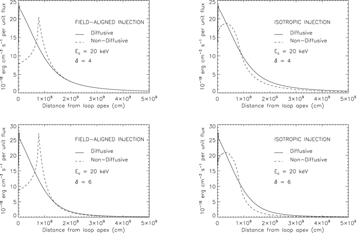
Figure 1. Comparison of heating profiles for E c = 20 keV and n = 1011 cm−3. The solid line in each panel represents the heating in the diffusional propagation. The dashed lines represent the heating in the deterministic model for a one-dimensional (field-aligned injection) model (left panel) and for a model with isotropic injection in a hemisphere (right panel).
Download figure:
Standard imageHigh-resolution image
For an anisotropic injection of electrons (or even an isotropic injection so that electrons proceed away from the injection point in separate hemispheres), a return current is rapidly established by the thermal electrons in the target plasma in order to effect charge and current neutralization (see Knight & Sturrock 1977; Emslie 1980; Spicer & Sudan 1984; Holman 1985; Larosa & Emslie 1989; van den Oord 1990; Zharkova et al. 1995; Zharkova & Gordovskyy 2005, 2006; Battaglia & Benz 2008; Codispoti et al. 2013). Driving this return current through the finite resistivity of the ambient medium results in an ohmic energy deposition rate
where the return current density is
For a local Ohm’s law , with scalar resistivity η, we thus have
The form of F(E, z) in this expression should, of course, be evaluated (or computed) self-consistently using both collisional and return current losses. However, as a first approximation, we can use the collisional diffusion result (19) for F(E, z) (this will be justified a posteriori below). Reversing the order of integration, we obtain
so that
The corresponding deterministic (nondiffusive) field-aligned injection result (e.g., Knight & Sturrock 1977; Emslie 1980) is obtained by using the form (21) for F(E, z) in Equation (42):
which simply reflects the conservation of particle flux down to depth , after which electrons are progressively “lost” from the beam. Thus, for such a nondiffusive field-aligned injection model,
Overall, the effect of diffusion is to reduce the anisotropy in the electron phase-space distribution function and thus reduce the magnitude of the return current and in turn the amount of ohmic heating. Figure 2 compares the ohmic heating profiles (in units of ) in the diffusive and field-aligned deterministic models. Including diffusion reduces the return current heating rate by a factor of about two to three near the injection point, and by over an order of magnitude near the point where electrons at the cutoff energy E c start to be lost from the beam.
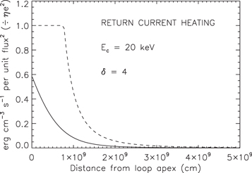
Figure 2. Comparison of return current ohmic heating profiles for E c = 20 keV and δ = 4. The solid line represents the heating in the diffusional propagation, while the dashed line represents the heating in the deterministic field-aligned injection model. The units of the heating are per unit squared injected particle flux , and are also scaled by the quantity η _e_2.
Download figure:
Standard imageHigh-resolution image
We can now justify a posteriori the use of the collision-dominated expression for F(E, z) in the calculation of the return current heating rate. An upper limit to the maximum return current heating rate is obtained by setting z = 0 in Equation (46):
To compare this with the maximum heating rate in the collisional model, we use the result (25) for the deterministic model at , since Figure 1 shows that the maximum heating rate in the diffusional model is similar. This allows us to calculate the ratio of the maximum return current ohmic heating to collisional heating:
Although electron transport properties such as thermal conductivity and resistivity can be altered in the presence of additional noncollisional processes, e.g., angular scattering off, for example, magnetic inhomogeneities (e.g., Bian et al. 2016), for consistency with the assumed collision-dominated transport we use the Spitzer (1962) expression
for the resistivity η. With this, Equation (48) becomes
where we have set δ = 4. Substituting E c = 20 keV = 3.2 × 10⁻⁸ erg, K, and cm−3 gives
Even for a large flare with s−1 and cm2, this gives . This ratio is even smaller in the diffusional model: although the maximum collisional heating rates in the diffusional and deterministic models are comparable (Figure 1), return current losses are significantly reduced relative to those in the deterministic model (Figure 2). We therefore see that return current ohmic losses are significantly less than collisional losses, so that the evolution of F(E, z) is controlled primarily by collisions. Thus the use of a collisional form for F(E, z) in determining the approximate return current losses is justified a posteriori.
Modeling of energy deposition by injected electron beams in solar flares previously assumed a directional beam accelerated in a point source and directed downward to the chromosphere where it was stopped collisionally. However, the need to include angular diffusion due to collisions in the physics of electron transport (Bian et al. 2017) results in significantly changed profiles for the electron flux versus depth and hence for the profile Q(z) of heat deposition versus depth. The resulting cold target heating function can, however, be adequately modeled simply by using a deterministic transport model with isotropic injection in the downward hemisphere (see the right panels of Figure 1). The effects on ohmic return current heating are more severe; the significantly greater level of isotropization of the injected electrons caused by enhanced pitch-angle scattering reduces the magnitude of the associated current, resulting in a reduction of up to an order of magnitude in the ohmic heating rate associated with the neutralizing return current.
This treatment can be extended to include noncollisional pitch-angle scattering of electrons in flaring loops (Kontar et al. 2014; Musset et al. 2018). In a future work, we will use these modified heating functions to determine the hydrodynamic response (Allred et al. 2015) of the solar atmosphere to the electron energy input. This will in turn allow us to construct velocity differential emission measure (Newton et al. 1995) profiles with which to compare observations of shifted and broadened soft X-ray and EUV spectral lines, with the ultimate goal of more meaningfully constraining the processes of nonthermal electron acceleration and transport during solar flares.
N.H.B. and A.G.E. were supported by grant NNX17AI16G from NASA’s Heliophysics Supporting Research program. E.P.K. was supported by a STFC consolidated grant ST/P000533/1.