Temporally Resolved Type III Solar Radio Bursts in the Frequency Range 3–13 MHz (original) (raw)
2041-8205/974/1/L18
Abstract
Radio observations from space allow to characterize solar radio bursts below the ionospheric cutoff, which are otherwise inaccessible, but suffer from low, insufficient temporal resolution. In this Letter we present novel, high-temporal resolution observations of type III solar radio bursts in the range 3–13 MHz. A dedicated configuration of the Radio and Plasma Waves (RPW) High Frequency Receiver (HFR) on the Solar Orbiter mission, allowing for a temporal resolution as high as ∼0.07 s (up to 2 orders of magnitude better than any other spacecraft measurements), provides for the very first time resolved measurements of the typical decay time values in this frequency range. The comparison of data with different time resolutions and acquired at different radial distances indicates that discrepancies with decay time values provided in previous studies are only due to the insufficient time resolution not allowing to accurately characterize decay times in this frequency range. The statistical analysis on a large sample of ∼500 type III radio bursts shows a power low decay time trend with a spectral index of −0.75 ± 0.03 when the median values for each frequency are considered. When these results are combined with previous observations, referring to frequencies outside the considered range, a spectral index of −1.00 ± 0.01 is found in the range ∼0.05–300 MHz, compatible with the presence of radio-wave scattering between 1 and 100 _R_☉.
Export citation and abstractBibTeXRIS
Solar type III radio bursts are among the most common impulsive radio emissions in the Universe. They are characterized by a rapid drift in time toward lower frequencies (f). The commonly accepted mechanism for the generation of type III radio bursts includes nonlinear wave coupling involving Langmuir waves generated by a “bump-on-tail instability” triggered by energetic electron beams. These are produced at the Sun during a flare and propagate through the plasma of the corona and the interplanetary medium with subluminal speed, typically 0.3–0.1_c_ (where c is the light speed). As the electrons move away from the Sun they encounter a decreasing electron density _n_e, and the Langmuir waves, emitted at the local plasma frequency _f_pe proportional to _n_e, generate radio waves at progressively decreasing frequencies as a function of the heliocentric distance. Type III radio bursts are observed over a wide range of frequencies ranging from about ∼500 MHz down to tens of kHz close to 1 au, corresponding to a wide range of heliocentric distances. The nonlinear coupling between Langmuir waves produces electromagnetic radiation near _f_pe, known as fundamental emission, or 2_f_pe, referred to as harmonic emission (see, e.g., S. Suzuki & G. A. Dulk 1985; M. Pick & N. Vilmer 2008, for reviews).
Density fluctuations along the path of the solar radio waves can strongly affect the propagation and the properties of the detected type III bursts. Scattering of radio waves on random density irregularities has long been recognized as an important process for the interpretation of radio source sizes (e.g., J. L. Steinberg et al. 1971), positions (e.g., A. D. Fokker 1965; R. T. Stewart 1972), directivity (e.g., G. Thejappa et al. 2007; X. Bonnin et al. 2008; M. J. Reiner et al. 2009), and intensity-time profiles (e.g., V. Krupar et al. 2018). In particular, due to the scattering, the intensity-time profiles for a fixed frequency (hereafter “light curves”) show typical features. (i) The light curve of a radio burst is characterized by a very fast rising phase followed by a long-lasting exponential decrease (e.g., L. G. Evans et al. 1973). Although at frequencies greater than 100 MHz the exponential decay can be also attributed to the emission process (e.g., B. Li et al. 2008), this is not the case for frequencies of the order of 10 MHz (H. Ratcliffe et al. 2014). At lower frequencies, indeed, the behavior of the decay phase is explained as the effect of the scattering of the radio waves by electron density inhomogeneities (see e.g., G. P. Zank et al. 2024) as they propagate from the source to the detector (V. Krupar et al. 2018; E. P. Kontar et al. 2019). The contributions to the rise phase are less clear, although radio scattering seems to play an important role (N. Chrysaphi et al. 2024). (ii) Since propagation effects are stronger when the frequency of the radio waves is close to the local _f_pe (e.g., J. L. Steinberg et al. 1971), lower frequencies scatter more than higher frequencies, thanks to the density scale heights being larger at larger heliocentric distances. This means that low-frequency radio photons, which undergo stronger scattering, disperse more compared to higher-frequency waves, giving rise to broader light curves with longer decay phases. This explains the relationship of inverse proportionality between decay time and frequency observed in all the data (e.g., J. K. Alexander et al. 1969; H. Alvarez & F. T. Haddock 1973; C. H. Barrow & A. Achong 1975; V. Krupar et al. 2018; H. A. S. Reid & E. P. Kontar 2018; E. P. Kontar et al. 2019; N. Chrysaphi et al. 2024).
Since decay times are directly related to the radio-wave scattering, their analysis and characterization can provide useful information about the strength and anisotropy of the scattering process (E. P. Kontar et al. 2019; X. Chen et al. 2020; A. A. Kuznetsov et al. 2020) and the level of density fluctuations (e.g., V. Krupar et al. 2018, 2020). By comparing radio burst properties over a large range of frequencies with advanced radio-wave propagation simulations, E. P. Kontar et al. (2019) showed that anisotropic scattering is required to reproduce the radio burst observations (decay time and source size), with the strongest scattering occurring perpendicular to the magnetic field direction, a result confirmed by multiple other studies (X. Chen et al. 2020; A. A. Kuznetsov et al. 2020; S. Musset et al. 2021; E. P. Kontar et al. 2023).
The plot of the decay time as a function of frequency, over the range ∼0.1–300 MHz (E. P. Kontar et al. 2019), obtained by combining various observations, shows two relevant features:
- (1)
The best fit of the decay time τ as a function of frequency f in MHz, assuming a f_−_β dependence is - (2)
A data gap is present between 3 and 13 MHz due to the lack of temporally resolved measurements. This gap represents a clear separation between measurements made from space and those made by radio observatories on ground.
Studies from the 70 s (T. R. Hartz 1964a; A. Boischot 1967) measured type III decay times in the 2–10 MHz (from the Alouette I spacecraft; time resolution 18 s (T. R. Hartz 1964b)) and 8–36 MHz (from the sweep frequency interferometer at the High Altitude Observatory Boulder; time resolution 4 s (A. Boischot et al. 1960)) finding dependency at τ ∝ _f_−0.98 and _f_−0.8, respectively. More recent studies, involving Parker Solar Probe (PSP) data, found different spectral indices: V. Krupar et al. (2020) found β = 0.5 s in the frequency range 0.5–10 MHz, while I. C. Jebaraj et al. (2023) detected β = 0.73 s in the range ∼1–20 MHz when a 3.5 s time resolution is set. We note that I. C. Jebaraj et al. (2023) used an exponentially modified Gaussian fit to derive smoother type III profiles and to calculate the decay time. Since the expected decay time in the frequency range considered here is of the order of 1–10 s, measurements with a time resolution of less than 1 s are therefore needed to accurately resolve the decay phase from the type III profiles. It is thus interesting to investigate whether the spread of the power-law exponents in previous studies could be due to the insufficient temporal resolution of these measurements.
The range 3–13 MHz, roughly corresponding to the radial belt 2–5 _R_☉ (according to the density model by E. C. J. Sittler & Guhathakurta 1999), represents a sort of boundary layer for several processes occurring in the interplanetary space. First, in this range of radial distances, the solar wind becomes supersonic behind the sonic critical point (S. R. Cranmer et al. 2023). At the same time, beyond about 5–7 _R_☉ the coronal plasma density varies as _r_−2, while its decrease is faster below it (see, e.g, E. C. J. Sittler & Guhathakurta 1999). Finally, the median radio flux density of type III radio bursts shows a maximum around 2 MHz, in the radial range 2–10 _R_☉, whose explanation is still to be found (V. Krupar et al. 2014; K. Sasikumar Raja et al. 2022). It is clear that filling the gap between 3 and 13 MHz with temporally resolved measurements is important to better understand the dynamics of this region of interplanetary space. In particular, accurate decay time measurements in this frequency range are needed to confirm the expected trend and characterize through observational data the scattering in the radial distance belt between 2 and 5 _R_☉ that currently remains unexplored.
From the instrumental point of view, the requirements for this kind of measurement are conceptually easy to achieve:
- (1)
These measurements have to be made from space as the Earth’s ionosphere partially reflects and absorbs the signals in this low-frequency range. - (2)
A relatively high time resolution is needed to properly sample signals with expected decay times of the order of 1–10 s.
The second point is not always easy to achieve since instruments on spacecraft are exploited for the widest possible variety of studies, and more general configurations that enable broad spectrum measurements are generally preferred. Five spacecraft currently orbiting in the interplanetary space would in principle be able to perform radio measurements in the frequency range of interest (the name of the receiver is in parentheses): Solar Orbiter (SO; Radio and Plasma Waves, RPW), PSP (FIELDS), STEREO-A (SWAVES), WIND (WAVES), and CHANG’E4-Queqiao (NCLE; Karapakula et al. 2024). Although the receivers of these missions are highly configurable, nominal configurations that usually involve measurements over much wider frequency ranges to maximize the scientific impact and over longer integration times to minimize noise are characterized by time resolutions of the order of seconds. It is clear that a dedicated configuration allowing an accurate measurement of the decay times in the 3–13 MHz range is necessary.
In this Letter we present for the first time high time-resolution measurements of type III burst decay times in the 3–13 MHz range by the High Frequency Receiver (HFR; M. Maksimovic et al. 2021; A. Vecchio et al. 2021) of the RPW instrument (M. Maksimovic et al. 2020) on board SO (D. Müller et al. 2020; I. Zouganelis et al. 2020). These measurements, covering about 13 months of observation, were obtained by a dedicated configuration of the HFR receiver that allowed acquisition of a light curve with a sample time of 0.07 s with an average value of ∼0.18 s. The achieved sample time is ∼50 times better than what PSP obtained during the sixth close encounter (enhanced temporal resolution of 3.5 s) and ∼200 times better than STEREO and WIND spacecraft. For NCLE, only commissioning data are currently available and they do not include measurements of type III bursts.
HFR is a sweeping receiver providing electric power spectral densities from 375 kHz up to 16 MHz with a maximum number of 321 frequency bins. The spectral properties of the measured signals are computed on board where the voltage power spectral density is sampled and transmitted on ground. HFR works only in the dipole mode, namely, the potential difference between couples of antennas is measured. A large variety of configurations, characterized by frequency range, number of frequency bins, and temporal and spectral resolutions, etc., are programmable in a series of operating modes optimized for specific analyses (M. Maksimovic et al. 2020). In its nominal configurations HFR makes measurements on 50 frequency bins. In the nominal burst mode, the one between the two nominal modes with the highest time resolution, this corresponds to a time sampling of each individual HFR spectrum of about 6 s. It is clear that such a sampling time is not enough to carry out the decay time measurements described above, and an ad hoc configuration is needed. For this purpose, starting from 2022 December 20, HFR was initially configured to acquire five frequency bins [3.225, 5.075, 6.875, 10.025, 12.225] MHz for ten times followed by a sweep on 50 frequency bins on the full HFR band between 0.425 and 16.325 MHz including the five frequencies above. Unfortunately, after a few rounds of measurements it was realized that the bins at 5.075 and 10.025 MHz are extremely noisy, due to interference from the platform (M. Maksimovic et al. 2021), and do not allow for a proper measurement of the light curves of type III bursts. It was therefore decided to replace these frequencies with 5.225 and 10.125 MHz. The final set of five frequency bins, effective from 2023 February 28, is [3.225, 5.225, 6.875, 10.125, 12.225] MHz. Although not optimal in terms of temporal resolution, the choice to have a long sweep on 50 frequencies is related to the possibility of obtaining spectrograms with a large enough number of points to produce daily dynamic spectra with sufficient resolution. The chosen HFR configuration, including performing an average on the lowest possible number of spectra (16) and measuring at only one sensor V1–V2, allows to reach, for each of the five chosen frequencies, a time resolution of ∼0.07 s for ten times followed by an acquisition between ∼0.5 and ∼0.8 s, according to the frequency, due to the long sweep. Figure A1 in Appendix A shows an example of the HFR frequency sweep as a function of time for the receiver configuration described above.
In this study the HFR power spectral densities from calibrated level 2 (L2) data were considered from 2022 December 20 to 2024 January 21 (the time interval when the HFR configuration described above was kept active). Although L2 data are only calibrated at the receiver level ( is expressed in physical units V2 Hz−1), this does not affect the calculation of the decay time, which, at a fixed frequency, only depends on the relative amplitudes at each time that do not change when the effects of antennas are included. The rising and decay phases of the type III profile are clearly visible in Figure 1, where the light curves at four frequencies are shown for a type III burst observed by HFR. Further examples are shown in Appendix A (Figures A2–A4).
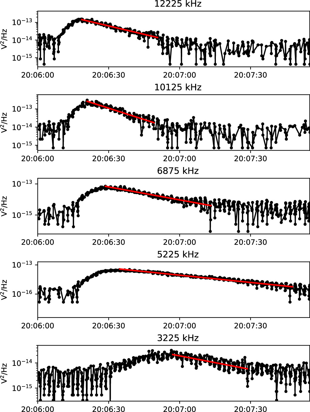
Figure 1. Light curves of the radio flux density measured by SO/RPW/HFR at five frequency channels during a type III burst on 2023 November 26. Red lines show the results of the decay time fitting.
Download figure:
Standard imageHigh-resolution image
In the analyzed data set, obtained on a daily basis, type III bursts are identified by looking at the light curves for the five considered frequencies. First the occurrence of a peak in the spectrum, possibly indicating a type III burst, is visually checked at the lowest frequency 3.225 MHz. The same peak is automatically sought at the other four frequencies in a time window 60 s before and 150 s after the peak at 3.225 MHz. The decay time τ is then obtained, for each frequency, by fitting the data points through an exponential function (J. K. Alexander et al. 1969; M. Aubier & A. Boischot 1972; H. Alvarez & F. T. Haddock 1973; C. H. Barrow & A. Achong 1975; V. Krupar et al. 2018; A. Vecchio et al. 2021) of the form
after removing the background. The left and right limits of the fitting interval are chosen as the point corresponding to the 0.95 of the maximum and the last value above the background, calculated as the median value of intensity over daily data. Although the necessity to evaluate τ with functions other than a single exponential has recently been demonstrated (N. Chrysaphi et al. 2024), in this Letter we preferred to use the classical approach to make a consistent comparison with the results found in the literature. An example of the result of the fitting procedure is shown in Figure 1.
By routinely analyzing the considered HFR daily data we were able to characterize the decay time for several events at the five recorded frequencies. The number of considered events for each frequency is displayed in Table A1. Decay time values were only selected according to the goodness of fit: only τ values coming out of converging fits with associated _R_2 values greater than 0.85 were considered. Figure 2(a) shows the histograms of τ for the five considered frequencies. The statistical distributions confirm that, on average, τ increases with decreasing frequency. This is a well-known property of the type III decay time due to the greater effectiveness of the radio-wave scattering at lower frequencies. The distributions of τ appear skewed, with quite long tails more pronounced for lower frequencies. The origin of the tail in the distribution lies in the blind selection of events only made according to the goodness of fit. At this stage, no visual selection was made to remove, for example, events characterized by multiple peaks for which the exponential fit, although converging from a purely mathematical point of view, has no clear physical meaning and can give rise to higher τ values. The results from the visually-selected data subset are shown in Figure 2(b), as discussed below.
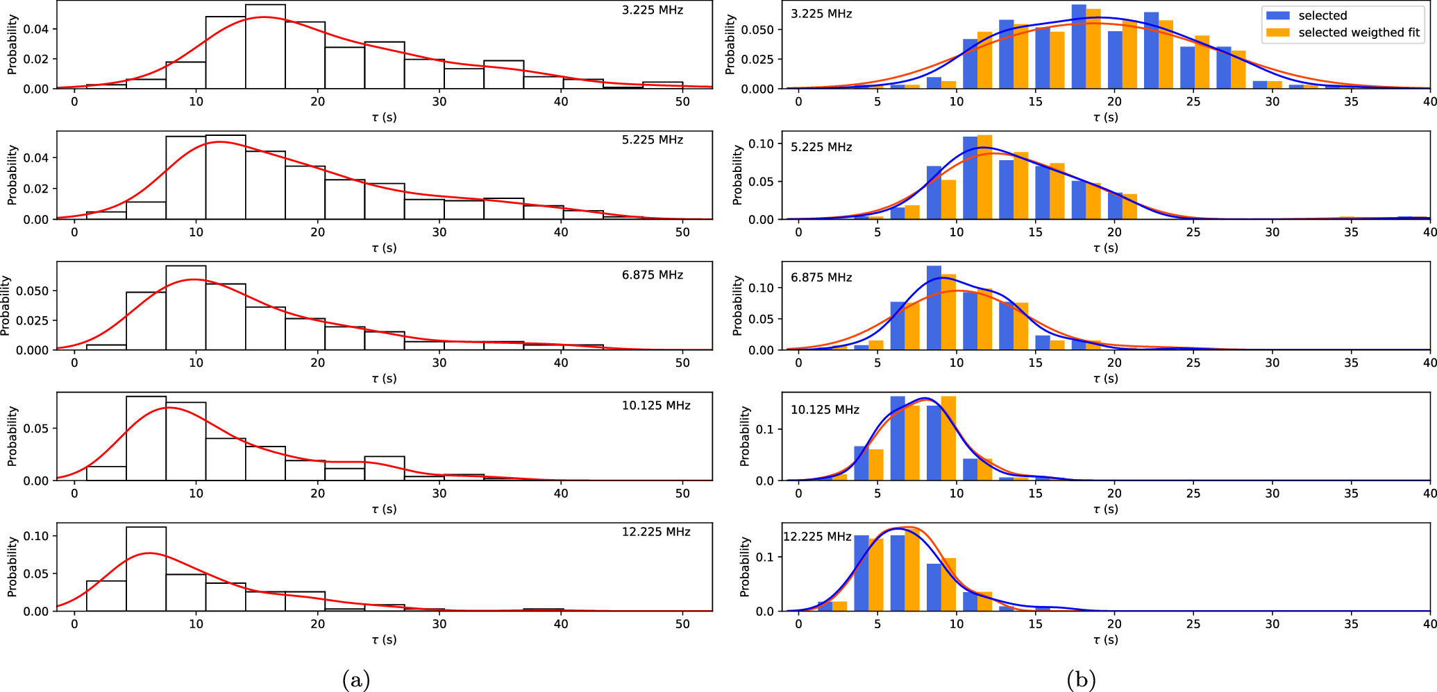
Figure 2. Histograms of the decay times obtained from the full data set (a) and from the visually selected type III burst subset (b) for unweighted (blue) and weighted (orange) fits, at the five considered frequencies. Red (a), blue, and orange (b) full lines represent the empirical probability density function, _P_emp(τ), estimated using the KDE approach and constructed from the histogram.
Download figure:
Standard imageHigh-resolution image
The properties of the distributions, median, and confidence interval provide statistically relevant information about the typical values of τ at each frequency. Moreover, to have an independent estimation for each frequency, the probability density function, _P_emp(τ), was empirically estimated using the kernel density estimation (KDE; see M. Rosenblatt 1956; E. Parzen 1962 for details), providing smooth and continuous functions (Figure 2(a), red line) by using a suitable kernel (B. W. Silverman 1986; P. Hall et al. 1992; D. W. Scott 1992). Gaussian kernels were considered, while the bandwidth was automatically detected through the “Scott rule of thumb” (D. W. Scott 1992), which works well for unimodal distributions. Figure 2(a) shows a very good agreement between the KDE curves and the decay time histogram.
The median values from each distribution together with the 5◦ and 95◦ percentiles are shown in Table A1. The value of τ corresponding to the maximum of each _P_emp(τ), used as another estimator of the characteristic τ, is also indicated in Table A1. Figure 3(a) shows the median values from the observed distributions as a function of the frequency. These values are well in agreement with the power law (Equation (1)) derived by fitting type III burst decay time measurements from both ground- and space-based data (E. P. Kontar et al. 2019).
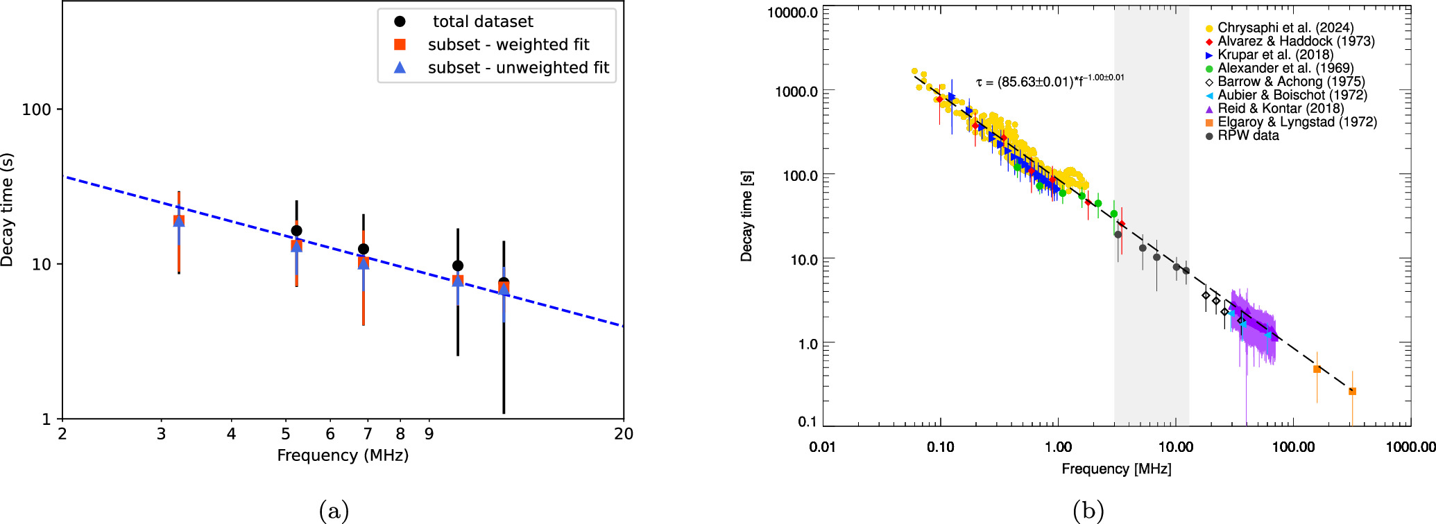
Figure 3. (a) Decay times for the five considered frequencies obtained as the median value from the observed distributions. Error bars represent the standard error. The dashed line shows the power-law function from Equation (1). (b) Median decay time values from the weighted fits on the type III bursts from the selected subset in the frequency range of 3–13 MHz (shaded region), superimposed on the data shown in Figure 10 of E. P. Kontar et al. (2019) and the newly added data from N. Chrysaphi et al. (2024). Error bars represent the standard error obtained from the observed distributions. The new best-fit function is also printed.
Download figure:
Standard imageHigh-resolution image
To check the validity of the blind selection of events, the same analysis has been applied to a subset of visually selected light curves corresponding to well-isolated type IIIs showing only a single peak. Table A2 shows the time of occurrence of the emission maximum, frequency of detection, and radial position of the selected type III bursts. The outcomes of this analysis have been compared to the results of weighted fits (using the intensity as weight) on all the type III burst profiles in the subset. The results are shown in Figures 2(b) and Table A3. Histograms from the subset appear less skewed with respect to the entire data set. This confirms that the fits on profiles with multiple peaks provide higher values of τ contributing to the longer tail of the histograms of the total data set (shown in Figure 2(a). Comparison of results from weighted and unweighted fits from the selected subset does not show significant differences on the histograms’ shape and median. Median, confidence interval, and KDE maxima from the selected subset are slightly lower than the ones from the full data set due to the higher degree of symmetry of the corresponding histograms. For the median tau values in Table A3, the weighted values are systematically slightly larger than the unweighted ones. This effect is due to the use of the intensity as a weight for the fit. Since higher intensity values close the maximum weigh more, they produce steeper fits than the unweighted case, and larger τ values are produced. The obtained results are robust with respect to the removal of noise, which is mainly due to the smaller number of photons collected because of the shorter acquisition time (see Figure 1). This was checked by applying two different filters, a median and a Wiener filter, to remove the noise from the data.
Figure 3(a) shows the median decay times for the five considered frequencies. Despite small differences, median values obtained for all three cases discussed above are in agreement with Equation (1) (Figure 3(a)), showing _R_2 values, obtained by comparing the model and the dependent variables when the linearized quantities are considered, of 0.76 (full data set) and 0.9 (for both weighted and unweighted data sets).
Figure 3(b) shows the median values derived by the weighted fits on the selected data subset, superimposed on the collection of type III burst decay time measurements presented by E. P. Kontar et al. (2019) and the data from N. Chrysaphi et al. (2024). The power-law fit has been revised by including the new RPW/HFR data discussed in this Letter and the measurements of N. Chrysaphi et al. (2024). The new best-fit function is
No significant changes with respect to Equation (1) (E. P. Kontar et al. 2019) were found, and the two functions can be considered equal within the limits of uncertainty. We note that the spectral index β = −1 does not change if all the detected τ, instead of the median values, are used for the fit. The addition of the new observations to the data set illustrated in E. P. Kontar et al. (2019) confirms that the dynamics of the radio-wave scattering in the 2–5 _R_☉ radial distance belt is the one expected from the trend obtained by measurements at higher and lower frequencies and that expected from numerical simulations of anisotropic scattering.
Unlike the peak intensity of radio emission showing a maximum at ∼2 MHz, decay times do not show any particular feature at the same frequencies.
3.1. Checking the Effects of Radial Distance and Time Resolution on the Decay Time Measurements
In this section we discuss whether our results can be affected by different plasma properties, due to different radial distances, and how the τ's spectral index is dependent on the time resolution of the data.
Figure 4 shows the measured decay times as a function of the radial distance of SO for the five considered frequencies. Radial distance does not correlate with decay time, consistently with the results of N. Chrysaphi et al. (2024). This indicates that the results shown in this Letter are robust with respect to the different radial distances of the measurements in the data sample.
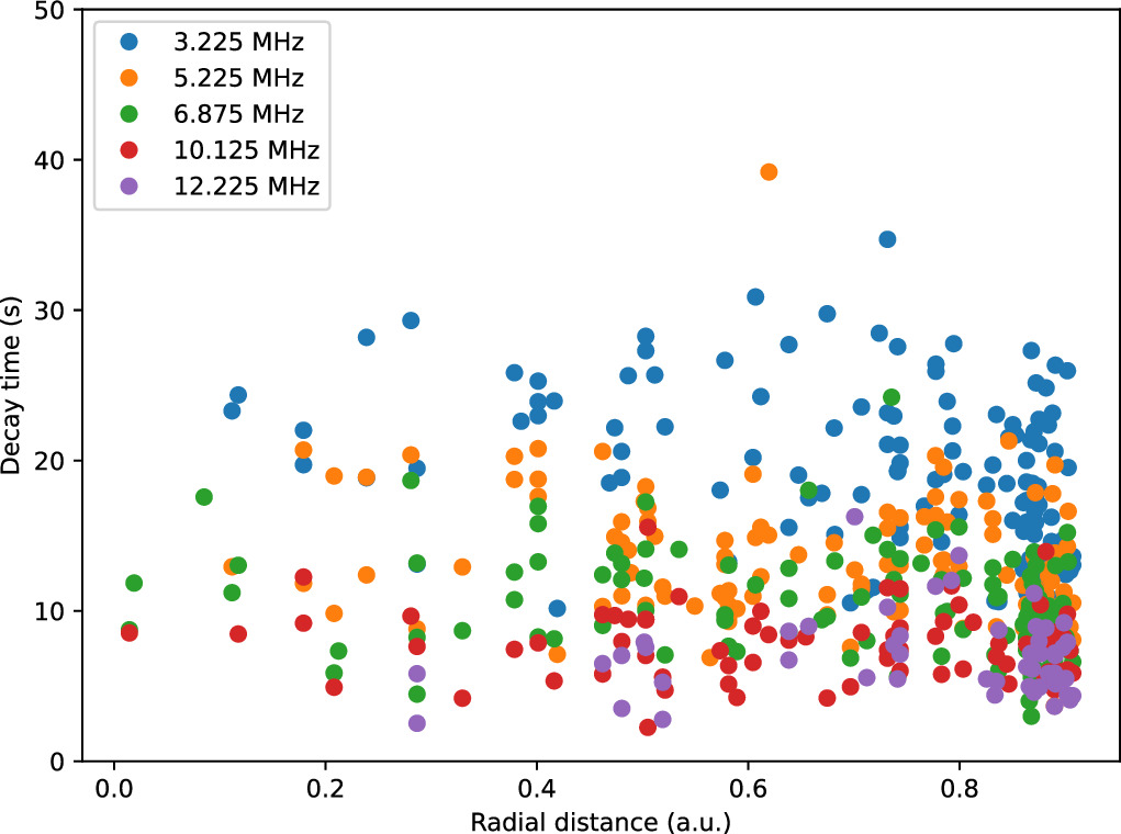
Figure 4. Decay time as a function of the radial distance for the five considered frequencies.
Download figure:
Standard imageHigh-resolution image
To study the effect of resolution on the measured decay times we reduced the time resolution of each light curve in our visually selected data set to the previously best resolution obtained from radio antennas in space (3.5 s from PSP). The same analysis above has been done on the reduced resolution data set. Histograms of the decay times from the new data set are shown in Figure A5 in Appendix A.
Panel (a) of Figure 5 shows a comparison of the decay times obtained by the original and reduced time resolution data set. This plot clearly highlights that at the lowest frequency of 3.225 MHz the results from the two data sets are comparable. The discrepancy between the two data sets increases, as expected, with increasing frequency since higher time resolution is needed to properly sample lower τ values. Panel (b) shows a comparison of the median values of the decay times as a function of frequency for the full (red) and reduced time resolution (black) data sets. While the full resolution data set well follows the trend of Equation (1), the reduced resolution data set strongly deviates from this at higher frequencies and shows a diverging _R_2 value. The power-law fit on the five points of both data sets provides an exponent of (−0.75 ± 0.03) for the original data set and (−0.19 ± 0.14) for the reduced resolution data set. The comparison of the decay time trends at different time resolutions shows that in the frequency range 3–13 MHz the discrepancy with Equation (1) increases when the time resolution of the data set decreases and a flatter trend is obtained. This behavior is confirmed when synthetic type III profiles are considered (Appendix B). Figure 5(b) also shows the median values of the decay times obtained from 3.5 s resolution PSP data for the events listed in I. C. Jebaraj et al. (2023). These decay times have been calculated by fitting PSP light curves with the same methodology followed throughout this Letter and described in Section 2. A spectral index β = −0.53 ± 0.03 is found. Also in this case the median values deviate from the trend of Equation (1) showing a significantly low _R_2 equal to 0.46 (compared to 0.76 and 0.9 for the full and visually selected data sets, respectively).
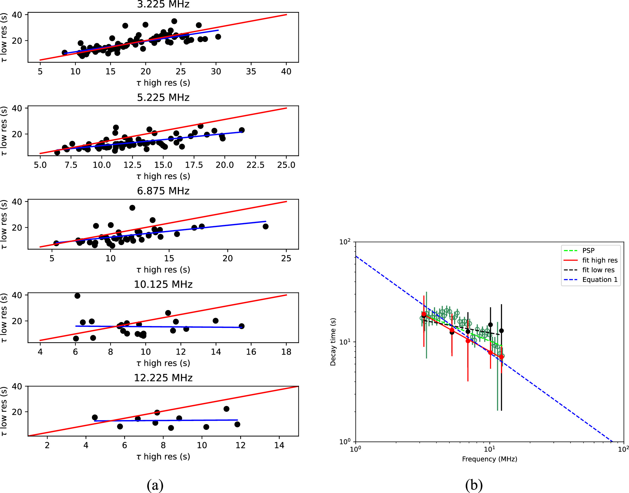
Figure 5. (a) Scatter plot of the decay times from the original data set at higher time resolution (_x_-axis) and reduced resolution (_y_-axis) for the five considered frequencies. The blue line represents the linear fit on the data, and the red line is the bisector. (b) Decay times for the five considered frequencies obtained as the median value from the observed distributions. Red: full time resolution data set; black: data set with time resolution reduced to 3.5 s; green: PSP data set with 3.5 s resolution. Error bars represent the standard error. The black, red, and lime lines correspond to the power-law fit on the respective five data points. The blue dashed line shows the power-law function from Equation (1).
Download figure:
Standard imageHigh-resolution image
These results show that the time resolution of the data set is the decisive factor for the proper measurement of decay times and the accurate determination of the law connecting τ to f in the frequency range considered here. The decay time calculations by V. Krupar et al. (2020) and I. C. Jebaraj et al. (2023) are not accurate enough since they are performed with a sampling time of the order of the expected decay time.
In this Letter we present measurements of type III burst decay time from high time-resolution radio data obtained using space-based instruments. The use of a special configuration of the HFR receiver of the RPW instrument on board SO allowed to sample spectra over five frequencies with a temporal resolution as high as 0.07 s (with an average resolution of ∼0.18 s), higher than all other available measurements. This, together with the availability of 11 months of measurements, allowed us to statistically characterize the τ behavior as a function of frequency in the range 3–13 MHz, based on a statistically large number of data points (see Table A1 and Table A3). Decay times, obtained though an exponential fit over the raw data, were calculated on the full sample of data and two subsamples of visually selected type III profiles, corresponding to well-isolated emissions whose decay times have been derived by weighted and unweighted fits. For the three data sets, the properties of the decay time distributions are in agreement, with the only evident difference being the presence of skewed distributions for the full sample. This is due to the presence of events characterized by multiple peaks in the full sample for which the exponential fit can give rise to higher τ values. When the median τ values are plotted as a function of frequency, a spectral index of −0.75 ± 0.03 is obtained by the performed power-law fit on the subsamples of visually-selected type III profiles (where light curves with multiple peaks were excluded). These results do not depend on the radial distance of the spacecraft, in agreement with the positional invariance demonstrated in N. Chrysaphi et al. (2024).
We also showed that the spectral index strongly depends on the time resolution of the radio spectra. Indeed, when the temporal resolution of the data is artificially reduced to 3.5 s, the discrepancy between median values from full and reduced resolution data increases with increasing frequency, since a higher time resolution is needed to properly sample lower decay times. A similar discrepancy with the full resolution RPW data set is observed when PSP data (3.5 s resolution) are considered. The spectral index of the median decay time for the reduced resolution data set and PSP data is −0.19 ± 0.14 and −0.53 ± 0.03, respectively, lower than the one from the full resolution data.
Finally we note that the decay time trend obtained from the full resolution measurements, unlike those from the reduced resolution RPW and PSP data, are compatible with the trend of Equation (1) obtained when several decay times are fitted in the range of ∼0.05–300 MHz.
All these results show that the time resolution of the data set is the decisive factor for the proper measurement of decay times and the accurate determination of the τ spectral index in the frequency range considered here. Discrepancies with the spectral indices obtained in previous studies (e.g., V. Krupar et al. 2018, 2020) do not arise by different radial distances during observations, but they are due to the different time resolutions of the data set. In particular, as shown in this Letter, the time resolution of the measurements used in previous works is insufficient to accurately characterize the decay time for frequencies higher than 6 MHz since the sampling time is comparable to the expected decay time. On the other hand, the special and unique configuration of SO/RPW/HFR, producing measurements with the highest temporal resolution ever obtained from space in the considered frequency range, allowed the decay time to be characterized in the range of 3–13 MHz with extreme accuracy. The combination of the decay times discussed in this Letter with the ones presented by E. P. Kontar et al. (2019) and N. Chrysaphi et al. (2024) provides a complete picture of the τ_–_f relationship in the range of 1–100 _R_☉ and allows to fill the long-standing gap in fully resolved observations of type III burst decay times in the frequency range of 3–13 MHz.
We acknowledge the two anonymous Reviewers for the useful discussions.
Solar Orbiter is a mission of international cooperation between ESA and NASA, operated by ESA. The RPW instrument has been designed and funded by CNES, CNRS, the Paris Observatory, the Swedish National Space Agency, ESA-PRODEX, and all the participating institutes. N. C. acknowledges funding support from the Initiative Physique des Infinis (IPI), a research training program of the Idex SUPER at Sorbonne Université. E. P. K. was supported via the STFC/UKRI grants ST/T000422/1 and ST/Y001834/1.
Appendix A presents Figures A1, A2, A3, A4, and A5, and Tables A1, A2, and A3.
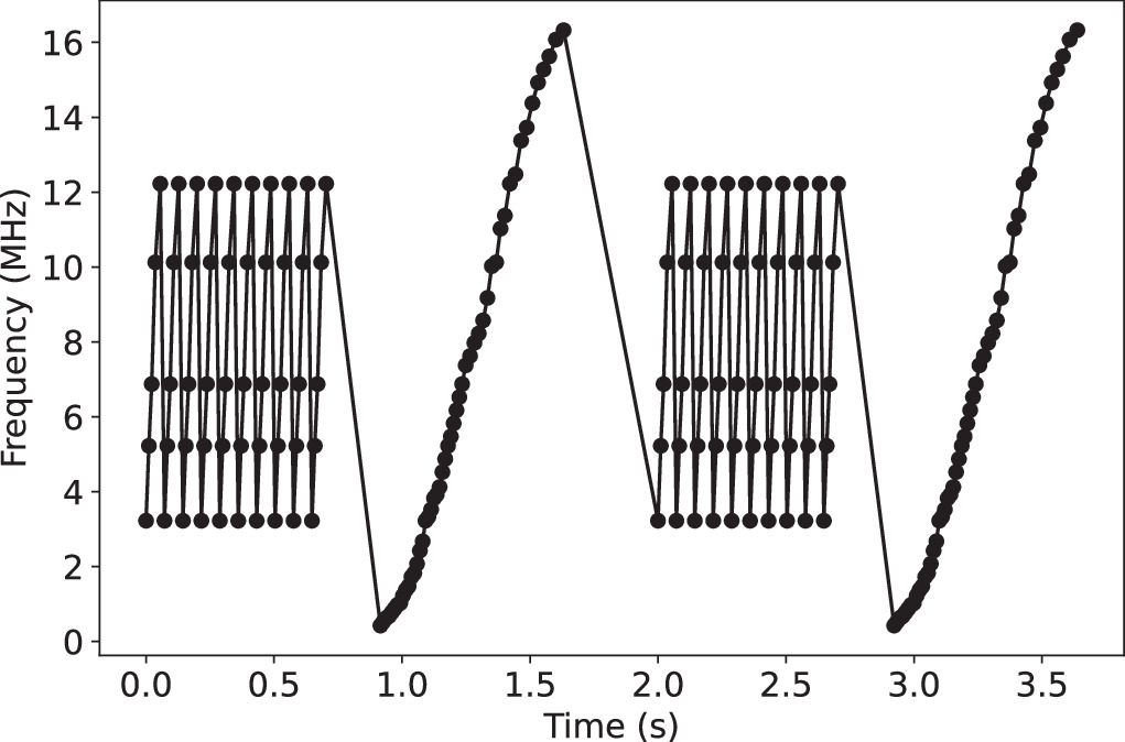
Figure A1. Example of the HFR frequency sweep as a function of time for the receiver configuration described in the main text. Time is measured in seconds from the beginning of the sweep.
Download figure:
Standard imageHigh-resolution image
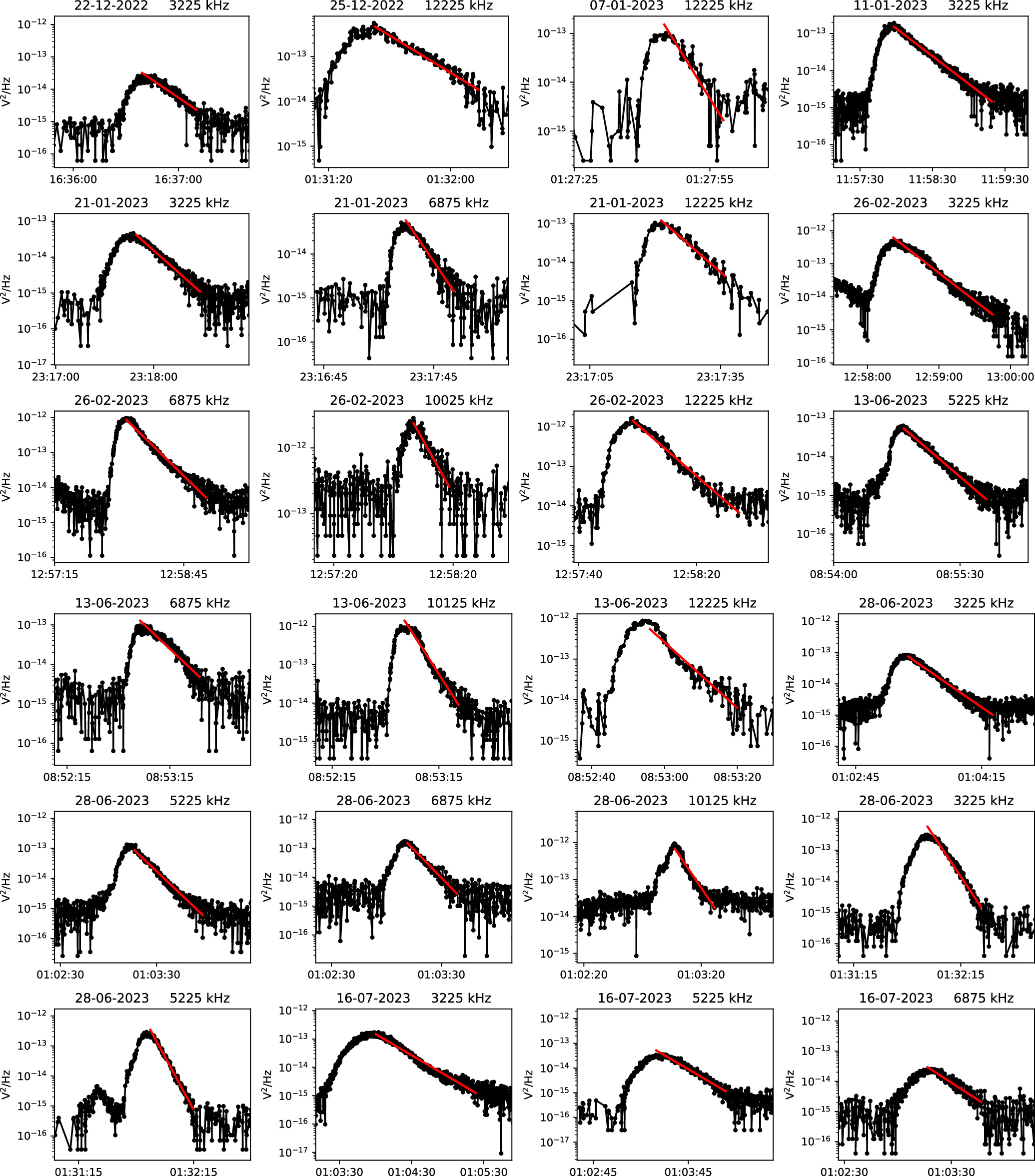
Figure A2. Light curves of the radio flux density measured by SO/RPW/HFR during a type III burst. Red lines show the results of the decay time fitting.
Download figure:
Standard imageHigh-resolution image
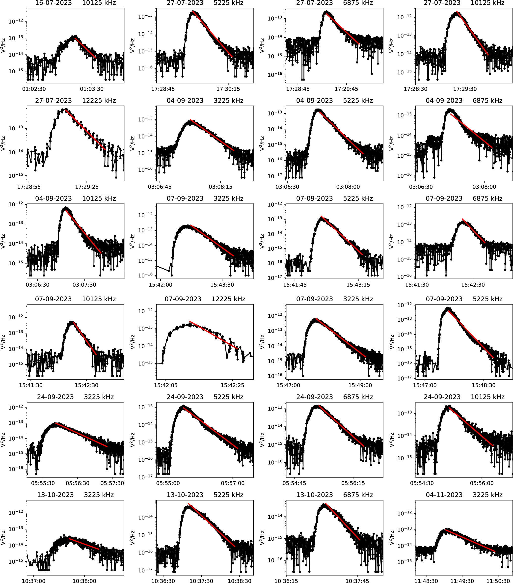
Figure A3. Light curves of the radio flux density measured by SO/RPW/HFR during a type III burst. Red lines show the results of the decay time fitting.
Download figure:
Standard imageHigh-resolution image
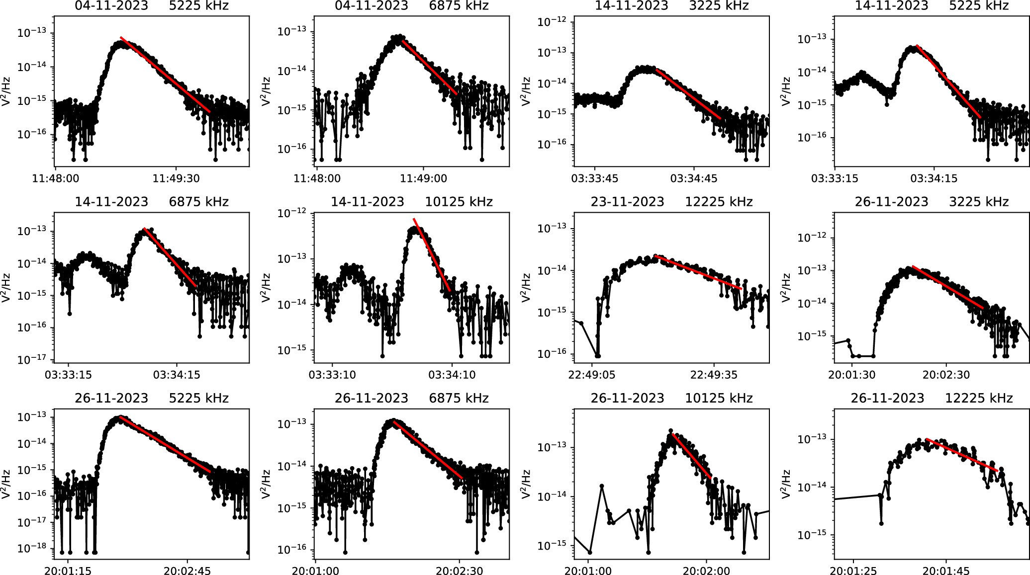
Figure A4. Light curves of the radio flux density measured by SO/RPW/HFR during a type III burst. Red lines show the results of the decay time fitting.
Download figure:
Standard imageHigh-resolution image
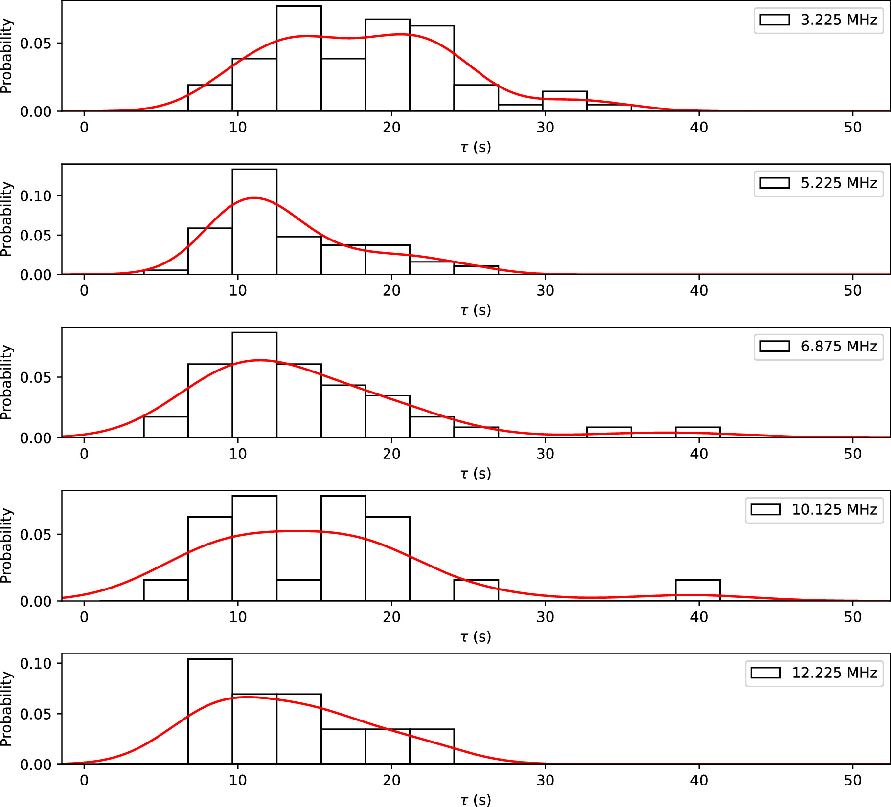
Figure A5. Histograms of the decay times obtained from the visually selected type III burst subset at the five considered frequencies when the time resolution has been reduced to 3.5 s. Red full lines represent the empirical probability density function estimated using the KDE approach and constructed from the histogram.
Download figure:
Standard imageHigh-resolution image
Table A1. Total Number of Measurements from the Full Data Set for Each Considered Frequency
| Frequency | Total Number of τ | med(τ) | Δ_τ_ | _τ_KDE |
|---|---|---|---|---|
| (MHz) | (s) | (s) | (s) | (s) |
| 3.225 | 349 | 19.06 | [9.98, 40.52] | 15.7 |
| 5.225 | 382 | 16.40 | [7.36, 37.07] | 11.9 |
| 6.875 | 220 | 12.49 | [5.62, 33.17] | 9.9 |
| 10.125 | 160 | 9.74 | [4.43, 25.13] | 7.75 |
| 12.225 | 107 | 7.57 | [2.60, 22.81] | 6.1 |
Note. med(τ) is the median value and Δ_τ_ represents the 5%–95% confidence interval obtained from each distribution. _τ_KDE corresponds to the maximum of the kernel density estimation of each distribution.
Download table as: ASCIITypeset image
Table A2. Time of Occurrence of the Emission Maximum, Frequency of Detection, and Radial Position of the Visually Selected Subset of Type III Bursts
| Date | Time | Frequency | Radial Distance |
|---|---|---|---|
| (UT) | (UT) | (kHz) | (au) |
| 20/12/2022 | 04:08:59 | 3225 | 0.86 |
| 20/12/2022 | 04:08:59 | 6875 | 0.86 |
| 21/12/2022 | 03:51:00 | 3225 | 0.86 |
| 21/12/2022 | 03:51:00 | 6875 | 0.86 |
| 21/12/2022 | 03:51:00 | 12225 | 0.86 |
| 21/12/2022 | 04:53:00 | 6875 | 0.86 |
| 21/12/2022 | 05:33:59 | 3225 | 0.86 |
| 22/12/2022 | 12:57:59 | 6875 | 0.86 |
| 22/12/2022 | 16:36:00 | 3225 | 0.86 |
| 22/12/2022 | 16:36:00 | 6875 | 0.86 |
| 22/12/2022 | 18:39:00 | 3225 | 0.86 |
| 22/12/2022 | 18:39:00 | 6875 | 0.86 |
| 22/12/2022 | 19:57:59 | 3225 | 0.86 |
| 22/12/2022 | 19:58:00 | 6875 | 0.86 |
| 24/12/2022 | 04:10:59 | 3225 | 0.87 |
| 24/12/2022 | 04:10:59 | 6875 | 0.87 |
| 24/12/2022 | 07:56:00 | 3225 | 0.87 |
| 24/12/2022 | 07:55:59 | 6875 | 0.87 |
| 25/12/2022 | 08:43:00 | 3225 | 0.87 |
| 25/12/2022 | 08:43:00 | 6875 | 0.87 |
| 25/12/2022 | 08:42:59 | 12225 | 0.87 |
| 27/12/2022 | 10:00:59 | 3225 | 0.87 |
| 28/12/2022 | 00:58:00 | 3225 | 0.87 |
| 28/12/2022 | 00:58:00 | 6875 | 0.87 |
| 28/12/2022 | 00:57:59 | 12225 | 0.87 |
| 28/12/2022 | 01:09:00 | 3225 | 0.87 |
| 28/12/2022 | 08:31:00 | 3225 | 0.87 |
| 01/01/2023 | 02:03:00 | 3225 | 0.87 |
| 01/01/2023 | 02:03:00 | 6875 | 0.87 |
| 01/01/2023 | 02:02:59 | 12225 | 0.87 |
| 01/01/2023 | 07:45:59 | 3225 | 0.87 |
| 02/01/2023 | 22:52:00 | 3225 | 0.87 |
| 06/01/2023 | 21:59:59 | 3225 | 0.87 |
| 06/01/2023 | 22:00:00 | 6875 | 0.87 |
| 07/01/2023 | 00:10:00 | 6875 | 0.87 |
| 07/01/2023 | 00:10:00 | 12225 | 0.87 |
| 07/01/2023 | 01:37:59 | 3225 | 0.87 |
| 07/01/2023 | 01:37:59 | 6875 | 0.87 |
| 07/01/2023 | 01:37:59 | 12225 | 0.87 |
| 07/01/2023 | 03🔞00 | 3225 | 0.87 |
| 07/01/2023 | 03🔞00 | 6875 | 0.87 |
| 08/01/2023 | 12:29:59 | 3225 | 0.86 |
| 08/01/2023 | 12:30:00 | 6875 | 0.86 |
| 08/01/2023 | 12:29:59 | 12225 | 0.86 |
| 09/01/2023 | 23:48:59 | 3225 | 0.86 |
| 09/01/2023 | 23:48:59 | 6875 | 0.86 |
| 09/01/2023 | 23:49:00 | 12225 | 0.86 |
| 11/01/2023 | 00:51:00 | 3225 | 0.86 |
| 11/01/2023 | 00:51:00 | 6875 | 0.86 |
| 11/01/2023 | 09🔞59 | 3225 | 0.86 |
| 11/01/2023 | 09🔞59 | 6875 | 0.86 |
| 11/01/2023 | 11:57:00 | 3225 | 0.86 |
| 15/01/2023 | 11:17:59 | 3225 | 0.85 |
| 16/01/2023 | 03:47:00 | 3225 | 0.85 |
| 16/01/2023 | 03:47:00 | 6875 | 0.85 |
| 16/01/2023 | 04:34:59 | 3225 | 0.85 |
| 20/01/2023 | 04:51:59 | 3225 | 0.83 |
| 20/01/2023 | 04:51:59 | 6875 | 0.83 |
| 21/01/2023 | 23:16:59 | 3225 | 0.83 |
| 21/01/2023 | 23:16:59 | 6875 | 0.83 |
| 21/01/2023 | 23:16:59 | 12225 | 0.83 |
| 30/01/2023 | 06:39:00 | 3225 | 0.79 |
| 05/02/2023 | 10:43:59 | 6875 | 0.76 |
| 09/02/2023 | 06:39:00 | 3225 | 0.74 |
| 09/02/2023 | 09:15:00 | 6875 | 0.74 |
| 09/02/2023 | 09:14:59 | 12225 | 0.74 |
| 09/02/2023 | 15:00:00 | 3225 | 0.74 |
| 09/02/2023 | 16:58:59 | 3225 | 0.74 |
| 10/02/2023 | 05:03:59 | 6875 | 0.73 |
| 12/02/2023 | 05:37:00 | 3225 | 0.72 |
| 13/02/2023 | 12:41:59 | 3225 | 0.71 |
| 13/02/2023 | 12:41:59 | 6875 | 0.71 |
| 14/02/2023 | 08:51:59 | 3225 | 0.71 |
| 14/02/2023 | 08:51:59 | 6875 | 0.71 |
| 14/02/2023 | 08:52:00 | 12225 | 0.71 |
| 19/02/2023 | 01:21:59 | 3225 | 0.68 |
| 19/02/2023 | 01:21:59 | 6875 | 0.68 |
| 21/02/2023 | 02:48:59 | 3225 | 0.66 |
| 21/02/2023 | 02:48:59 | 6875 | 0.66 |
| 23/02/2023 | 23:15:00 | 3225 | 0.65 |
| 23/02/2023 | 23:15:00 | 6875 | 0.65 |
| 23/02/2023 | 23:15:00 | 12225 | 0.65 |
| 26/02/2023 | 12:58:00 | 3225 | 0.63 |
| 26/02/2023 | 12:58:00 | 6875 | 0.63 |
| 26/02/2023 | 12:57:59 | 10125 | 0.63 |
| 26/02/2023 | 12:57:59 | 12225 | 0.63 |
| 26/02/2023 | 18:34:00 | 6875 | 0.63 |
| 26/02/2023 | 19:13:00 | 3225 | 0.63 |
| 26/02/2023 | 19:13:00 | 6875 | 0.63 |
| 26/02/2023 | 19:13:00 | 12225 | 0.63 |
| 01/03/2023 | 01:36:59 | 5225 | 0.61 |
| 03/03/2023 | 04:48:59 | 3225 | 0.60 |
| 03/03/2023 | 04:48:59 | 5225 | 0.60 |
| 03/03/2023 | 04:48:59 | 6875 | 0.60 |
| 18/03/2023 | 02:31:00 | 5225 | 0.50 |
| 18/03/2023 | 02:30:59 | 10125 | 0.50 |
| 18/03/2023 | 09:09:00 | 10125 | 0.50 |
| 18/03/2023 | 16:16:00 | 5225 | 0.50 |
| 20/03/2023 | 02:10:59 | 5225 | 0.48 |
| 21/03/2023 | 08:51:59 | 5225 | 0.48 |
| 21/03/2023 | 10:20:00 | 10125 | 0.48 |
| 21/03/2023 | 10:20:00 | 12225 | 0.48 |
| 23/03/2023 | 17:31:00 | 5225 | 0.46 |
| 23/03/2023 | 17:31:00 | 6875 | 0.46 |
| 23/03/2023 | 17:31:00 | 10125 | 0.46 |
| 23/03/2023 | 18:50:59 | 5225 | 0.46 |
| 23/03/2023 | 18:50:59 | 6875 | 0.46 |
| 23/03/2023 | 18:51:00 | 10125 | 0.46 |
| 23/03/2023 | 18:51:00 | 12225 | 0.46 |
| 27/03/2023 | 21:59:59 | 3225 | 0.41 |
| 27/03/2023 | 21:59:59 | 5225 | 0.41 |
| 30/03/2023 | 10:58:59 | 3225 | 0.37 |
| 30/03/2023 | 10:59:00 | 5225 | 0.37 |
| 30/03/2023 | 10:59:00 | 6875 | 0.37 |
| 30/03/2023 | 10:59:00 | 10125 | 0.37 |
| 30/03/2023 | 23:10:00 | 5225 | 0.37 |
| 30/03/2023 | 23:10:00 | 6875 | 0.37 |
| 04/04/2023 | 03:53:59 | 5225 | 0.28 |
| 04/04/2023 | 03:53:59 | 6875 | 0.28 |
| 04/04/2023 | 03:54:00 | 12225 | 0.28 |
| 04/04/2023 | 04:11:00 | 3225 | 0.28 |
| 04/04/2023 | 04:10:59 | 6875 | 0.28 |
| 04/04/2023 | 04:11:00 | 12225 | 0.28 |
| 04/04/2023 | 04:38:00 | 3225 | 0.28 |
| 04/04/2023 | 16:12:00 | 6875 | 0.28 |
| 04/04/2023 | 16:12:00 | 10125 | 0.28 |
| 06/04/2023 | 06:42:59 | 3225 | 0.23 |
| 06/04/2023 | 08:47:59 | 3225 | 0.23 |
| 06/04/2023 | 08:47:59 | 5225 | 0.23 |
| 06/04/2023 | 18:59:00 | 5225 | 0.23 |
| 07/04/2023 | 02:39:00 | 6875 | 0.21 |
| 03/05/2023 | 01:49:00 | 3225 | 0.47 |
| 03/05/2023 | 01:48:59 | 5225 | 0.47 |
| 03/05/2023 | 01:48:59 | 6875 | 0.47 |
| 03/05/2023 | 01:48:59 | 10125 | 0.47 |
| 31/05/2023 | 04:00:59 | 3225 | 0.78 |
| 31/05/2023 | 04:01:00 | 5225 | 0.78 |
| 31/05/2023 | 04:01:00 | 6875 | 0.78 |
| 10/06/2023 | 14:40:59 | 3225 | 0.84 |
| 10/06/2023 | 14:40:59 | 5225 | 0.84 |
| 10/06/2023 | 14:40:59 | 6875 | 0.84 |
| 10/06/2023 | 14:40:59 | 10125 | 0.84 |
| 14/06/2023 | 03:01:59 | 3225 | 0.86 |
| 14/06/2023 | 03:01:59 | 5225 | 0.86 |
| 24/06/2023 | 04:33:59 | 3225 | 0.88 |
| 25/06/2023 | 15:55:59 | 3225 | 0.88 |
| 25/06/2023 | 15:56:00 | 5225 | 0.88 |
| 27/06/2023 | 23:31:59 | 3225 | 0.88 |
| 27/06/2023 | 23:31:59 | 5225 | 0.88 |
| 28/06/2023 | 01:03:00 | 3225 | 0.88 |
| 28/06/2023 | 01:03:00 | 5225 | 0.88 |
| 28/06/2023 | 01:03:00 | 6875 | 0.88 |
| 28/06/2023 | 01:31:00 | 3225 | 0.88 |
| 28/06/2023 | 01:31:00 | 5225 | 0.88 |
| 28/06/2023 | 03:47:00 | 3225 | 0.88 |
| 28/06/2023 | 03:46:59 | 5225 | 0.88 |
| 28/06/2023 | 03:46:59 | 6875 | 0.88 |
| 28/06/2023 | 03:46:59 | 10125 | 0.88 |
| 28/06/2023 | 03:47:00 | 12225 | 0.88 |
| 28/06/2023 | 10:57:59 | 5225 | 0.88 |
| 28/06/2023 | 10:57:59 | 6875 | 0.88 |
| 28/06/2023 | 10:58:00 | 10125 | 0.88 |
| 28/06/2023 | 10:58:00 | 12225 | 0.88 |
| 29/06/2023 | 00:24:00 | 3225 | 0.89 |
| 29/06/2023 | 00:24:00 | 5225 | 0.89 |
| 29/06/2023 | 00:24:00 | 6875 | 0.89 |
| 29/06/2023 | 00:24:00 | 10125 | 0.89 |
| 29/06/2023 | 00:23:59 | 12225 | 0.89 |
| 29/06/2023 | 03:42:59 | 6875 | 0.89 |
| 29/06/2023 | 03:42:59 | 10125 | 0.89 |
| 29/06/2023 | 03:43:00 | 12225 | 0.89 |
| 01/07/2023 | 11:31:59 | 3225 | 0.89 |
| 02/07/2023 | 00:15:59 | 5225 | 0.89 |
| 02/07/2023 | 00:15:59 | 6875 | 0.89 |
| 02/07/2023 | 00:15:59 | 10125 | 0.89 |
| 02/07/2023 | 00:15:59 | 12225 | 0.89 |
| 03/07/2023 | 12:46:00 | 3225 | 0.89 |
| 03/07/2023 | 12:46:00 | 5225 | 0.89 |
| 04/07/2023 | 06:41:00 | 3225 | 0.89 |
| 04/07/2023 | 06:41:00 | 5225 | 0.89 |
| 07/07/2023 | 22:35:00 | 3225 | 0.88 |
| 07/07/2023 | 22:34:59 | 5225 | 0.88 |
| 08/07/2023 | 18:53:59 | 3225 | 0.88 |
| 08/07/2023 | 18:53:59 | 5225 | 0.88 |
| 08/07/2023 | 18:54:00 | 6875 | 0.88 |
| 08/07/2023 | 18:54:00 | 10125 | 0.88 |
| 10/07/2023 | 10:44:59 | 3225 | 0.88 |
| 10/07/2023 | 10:44:59 | 5225 | 0.88 |
| 10/07/2023 | 10:44:59 | 6875 | 0.88 |
| 10/07/2023 | 10:44:59 | 10125 | 0.88 |
| 10/07/2023 | 10:44:59 | 12225 | 0.88 |
| 12/07/2023 | 11:14:59 | 10125 | 0.88 |
| 14/07/2023 | 10:01:00 | 10125 | 0.87 |
| 14/07/2023 | 10:01:00 | 12225 | 0.87 |
| 16/07/2023 | 01:04:00 | 3225 | 0.87 |
| 16/07/2023 | 01:04:00 | 5225 | 0.87 |
| 16/07/2023 | 01:04:00 | 6875 | 0.87 |
| 16/07/2023 | 01:04:00 | 10125 | 0.87 |
| 16/07/2023 | 22:21:00 | 3225 | 0.87 |
| 16/07/2023 | 22:21:00 | 5225 | 0.87 |
| 16/07/2023 | 22:21:00 | 6875 | 0.87 |
| 18/07/2023 | 00:32:59 | 3225 | 0.86 |
| 18/07/2023 | 18:41:00 | 6875 | 0.86 |
| 18/07/2023 | 21:45:59 | 3225 | 0.86 |
| 18/07/2023 | 21:46:00 | 5225 | 0.86 |
| 19/07/2023 | 20:48:00 | 3225 | 0.86 |
| 19/07/2023 | 20:48:00 | 5225 | 0.86 |
| 19/07/2023 | 20:48:00 | 6875 | 0.86 |
| 19/07/2023 | 20:47:59 | 10125 | 0.86 |
| 19/07/2023 | 20:47:59 | 12225 | 0.86 |
| 20/07/2023 | 09:59:00 | 3225 | 0.86 |
| 20/07/2023 | 18:31:59 | 3225 | 0.86 |
| 20/07/2023 | 18:31:59 | 5225 | 0.86 |
| 20/07/2023 | 18:31:59 | 6875 | 0.86 |
| 24/07/2023 | 04:57:59 | 3225 | 0.84 |
| 24/07/2023 | 04:57:59 | 5225 | 0.84 |
| 24/07/2023 | 04:58:00 | 10125 | 0.84 |
| 27/07/2023 | 17:29:00 | 3225 | 0.83 |
| 27/07/2023 | 17:29:00 | 5225 | 0.83 |
| 27/07/2023 | 17:29:00 | 6875 | 0.83 |
| 27/07/2023 | 17:28:59 | 10125 | 0.83 |
| 27/07/2023 | 17:28:59 | 12225 | 0.83 |
| 03/08/2023 | 09:12:00 | 3225 | 0.80 |
| 03/08/2023 | 09:11:59 | 6875 | 0.80 |
| 03/08/2023 | 09:11:59 | 10125 | 0.80 |
| 03/08/2023 | 19:58:59 | 5225 | 0.80 |
| 03/08/2023 | 19:58:59 | 6875 | 0.80 |
| 05/08/2023 | 05:23:59 | 3225 | 0.79 |
| 05/08/2023 | 10:58:59 | 3225 | 0.79 |
| 07/08/2023 | 16:30:59 | 3225 | 0.78 |
| 07/08/2023 | 16:31:00 | 5225 | 0.78 |
| 07/08/2023 | 16:31:00 | 6875 | 0.78 |
| 07/08/2023 | 16:31:00 | 10125 | 0.78 |
| 07/08/2023 | 20:52:00 | 5225 | 0.78 |
| 07/08/2023 | 20:52:00 | 6875 | 0.78 |
| 08/08/2023 | 01:05:00 | 3225 | 0.77 |
| 08/08/2023 | 01:05:00 | 5225 | 0.77 |
| 08/08/2023 | 11:38:59 | 3225 | 0.77 |
| 08/08/2023 | 11:38:59 | 5225 | 0.77 |
| 10/08/2023 | 07:14:59 | 5225 | 0.76 |
| 10/08/2023 | 22:02:00 | 3225 | 0.76 |
| 10/08/2023 | 22:02:00 | 5225 | 0.76 |
| 14/08/2023 | 07:06:00 | 3225 | 0.74 |
| 14/08/2023 | 07:06:00 | 10125 | 0.74 |
| 14/08/2023 | 07:06:00 | 12225 | 0.74 |
| 14/08/2023 | 09:28:00 | 3225 | 0.74 |
| 14/08/2023 | 09:28:00 | 5225 | 0.74 |
| 14/08/2023 | 09:28:00 | 6875 | 0.74 |
| 14/08/2023 | 09:27:59 | 10125 | 0.74 |
| 14/08/2023 | 16:26:59 | 3225 | 0.74 |
| 14/08/2023 | 16:26:59 | 5225 | 0.74 |
| 14/08/2023 | 16:27:00 | 10125 | 0.74 |
| 14/08/2023 | 16:27:00 | 12225 | 0.74 |
| 14/08/2023 | 17:46:59 | 3225 | 0.74 |
| 14/08/2023 | 17:46:59 | 5225 | 0.74 |
| 14/08/2023 | 17:46:59 | 6875 | 0.74 |
| 14/08/2023 | 17:47:00 | 10125 | 0.74 |
| 15/08/2023 | 00:45:00 | 3225 | 0.73 |
| 15/08/2023 | 00:45:00 | 5225 | 0.73 |
| 15/08/2023 | 00:45:00 | 6875 | 0.73 |
| 15/08/2023 | 00:44:59 | 10125 | 0.73 |
| 15/08/2023 | 00:44:59 | 12225 | 0.73 |
| 16/08/2023 | 00:59:00 | 5225 | 0.73 |
| 16/08/2023 | 00:59:00 | 6875 | 0.73 |
| 16/08/2023 | 00:59:00 | 10125 | 0.73 |
| 16/08/2023 | 00:59:00 | 12225 | 0.73 |
| 16/08/2023 | 07:09:00 | 3225 | 0.73 |
| 16/08/2023 | 13:07:59 | 3225 | 0.73 |
| 16/08/2023 | 13:07:59 | 5225 | 0.73 |
| 16/08/2023 | 13:08:00 | 10125 | 0.73 |
| 16/08/2023 | 16:00:59 | 3225 | 0.73 |
| 16/08/2023 | 16:00:59 | 5225 | 0.73 |
| 16/08/2023 | 16:32:59 | 10125 | 0.73 |
| 20/08/2023 | 13:29:00 | 3225 | 0.70 |
| 20/08/2023 | 13:28:59 | 5225 | 0.70 |
| 20/08/2023 | 13:28:59 | 6875 | 0.70 |
| 20/08/2023 | 13:28:59 | 10125 | 0.70 |
| 20/08/2023 | 14:16:59 | 3225 | 0.70 |
| 20/08/2023 | 14:16:59 | 5225 | 0.70 |
| 21/08/2023 | 16:27:00 | 5225 | 0.70 |
| 21/08/2023 | 16:26:59 | 12225 | 0.70 |
| 24/08/2023 | 20:36:00 | 3225 | 0.68 |
| 24/08/2023 | 20:36:00 | 5225 | 0.68 |
| 25/08/2023 | 03:26:59 | 5225 | 0.67 |
| 25/08/2023 | 03:26:59 | 6875 | 0.67 |
| 25/08/2023 | 03:27:00 | 10125 | 0.67 |
| 25/08/2023 | 09:09:00 | 3225 | 0.67 |
| 25/08/2023 | 09:08:59 | 5225 | 0.67 |
| 28/08/2023 | 20:25:59 | 10125 | 0.65 |
| 29/08/2023 | 00:07:00 | 3225 | 0.64 |
| 29/08/2023 | 00:07:00 | 5225 | 0.64 |
| 02/09/2023 | 03:46:00 | 5225 | 0.61 |
| 02/09/2023 | 03:45:59 | 10125 | 0.61 |
| 03/09/2023 | 09:53:59 | 5225 | 0.61 |
| 03/09/2023 | 09:54:00 | 10125 | 0.61 |
| 03/09/2023 | 16:29:59 | 3225 | 0.61 |
| 03/09/2023 | 17:35:59 | 5225 | 0.61 |
| 04/09/2023 | 03:06:59 | 10125 | 0.60 |
| 04/09/2023 | 04:55:59 | 5225 | 0.60 |
| 04/09/2023 | 06:24:00 | 3225 | 0.60 |
| 04/09/2023 | 06:24:00 | 5225 | 0.60 |
| 04/09/2023 | 06:23:59 | 10125 | 0.60 |
| 06/09/2023 | 20:46:00 | 5225 | 0.58 |
| 06/09/2023 | 22:33:59 | 6875 | 0.58 |
| 06/09/2023 | 22:33:59 | 10125 | 0.58 |
| 07/09/2023 | 03:24:00 | 5225 | 0.58 |
| 07/09/2023 | 03:24:00 | 10125 | 0.58 |
| 07/09/2023 | 15:41:59 | 3225 | 0.58 |
| 07/09/2023 | 15:41:59 | 5225 | 0.58 |
| 07/09/2023 | 15:41:59 | 6875 | 0.58 |
| 07/09/2023 | 15:42:00 | 10125 | 0.58 |
| 07/09/2023 | 15:47:00 | 5225 | 0.58 |
| 07/09/2023 | 18:33:59 | 5225 | 0.58 |
| 07/09/2023 | 18:33:59 | 6875 | 0.58 |
| 08/09/2023 | 07:34:59 | 3225 | 0.57 |
| 08/09/2023 | 07:34:59 | 5225 | 0.57 |
| 08/09/2023 | 07:35:00 | 10125 | 0.57 |
| 14/09/2023 | 09:21:00 | 3225 | 0.52 |
| 14/09/2023 | 09:21:00 | 5225 | 0.52 |
| 14/09/2023 | 09:21:00 | 6875 | 0.52 |
| 14/09/2023 | 09:21:00 | 10125 | 0.52 |
| 15/09/2023 | 07:35:00 | 3225 | 0.51 |
| 15/09/2023 | 07:35:00 | 5225 | 0.51 |
| 16/09/2023 | 09:02:59 | 5225 | 0.50 |
| 16/09/2023 | 09:03:00 | 6875 | 0.50 |
| 16/09/2023 | 09:03:00 | 12225 | 0.50 |
| 18/09/2023 | 12:13:13 | 5225 | 0.48 |
| 18/09/2023 | 17:22:00 | 3225 | 0.48 |
| 18/09/2023 | 17:21:59 | 5225 | 0.48 |
| 18/09/2023 | 17:21:59 | 6875 | 0.48 |
| 18/09/2023 | 17:21:59 | 12225 | 0.48 |
| 18/09/2023 | 18:05:59 | 3225 | 0.48 |
| 18/09/2023 | 18:06:00 | 6875 | 0.48 |
| 19/09/2023 | 11:15:59 | 3225 | 0.46 |
| 23/09/2023 | 09:11:59 | 3225 | 0.41 |
| 23/09/2023 | 09:11:59 | 6875 | 0.41 |
| 23/09/2023 | 09:11:59 | 10125 | 0.41 |
| 24/09/2023 | 05:55:00 | 3225 | 0.40 |
| 24/09/2023 | 05:55:00 | 5225 | 0.40 |
| 24/09/2023 | 05:55:00 | 6875 | 0.40 |
| 24/09/2023 | 08:02:59 | 3225 | 0.40 |
| 24/09/2023 | 08:02:59 | 5225 | 0.40 |
| 24/09/2023 | 08:02:59 | 6875 | 0.40 |
| 24/09/2023 | 10:23:00 | 3225 | 0.40 |
| 24/09/2023 | 10:22:59 | 5225 | 0.40 |
| 24/09/2023 | 10:22:59 | 6875 | 0.40 |
| 24/09/2023 | 10:22:59 | 10125 | 0.40 |
| 24/09/2023 | 15:32:59 | 6875 | 0.40 |
| 25/09/2023 | 15:43:59 | 3225 | 0.38 |
| 28/09/2023 | 03:55:59 | 10125 | 0.32 |
| 28/09/2023 | 05:14:00 | 5225 | 0.32 |
| 28/09/2023 | 05:14:00 | 6875 | 0.32 |
| 03/10/2023 | 19:05:59 | 5225 | 0.20 |
| 03/10/2023 | 19:05:59 | 6875 | 0.20 |
| 03/10/2023 | 19:06:00 | 10125 | 0.20 |
| 03/10/2023 | 20:40:59 | 5225 | 0.20 |
| 04/10/2023 | 14:10:59 | 5225 | 0.17 |
| 04/10/2023 | 14:11:00 | 10125 | 0.17 |
| 04/10/2023 | 14:47:59 | 3225 | 0.17 |
| 04/10/2023 | 14:47:59 | 5225 | 0.17 |
| 04/10/2023 | 20:12:59 | 3225 | 0.17 |
| 04/10/2023 | 20:12:59 | 10125 | 0.17 |
| 06/10/2023 | 20:59:00 | 3225 | 0.11 |
| 06/10/2023 | 20:59:00 | 6875 | 0.11 |
| 06/10/2023 | 20:59:00 | 10125 | 0.11 |
| 07/10/2023 | 12:21:00 | 6875 | 0.08 |
| 09/10/2023 | 04:46:59 | 6875 | 0.01 |
| 10/10/2023 | 03:47:59 | 6875 | 0.01 |
| 10/10/2023 | 03:47:59 | 10125 | 0.01 |
| 13/10/2023 | 10:37:00 | 3225 | 0.11 |
| 13/10/2023 | 10:36:59 | 5225 | 0.11 |
| 13/10/2023 | 10:36:59 | 6875 | 0.11 |
| 19/10/2023 | 04:40:00 | 3225 | 0.28 |
| 19/10/2023 | 04:39:59 | 5225 | 0.28 |
| 19/10/2023 | 04:39:59 | 6875 | 0.28 |
| 19/10/2023 | 04:39:59 | 10125 | 0.28 |
| 29/10/2023 | 22🔞00 | 3225 | 0.48 |
| 29/10/2023 | 22🔞00 | 5225 | 0.48 |
| 29/10/2023 | 22:17:59 | 10125 | 0.48 |
| 30/10/2023 | 10:48:00 | 6875 | 0.50 |
| 30/10/2023 | 10:47:59 | 10125 | 0.50 |
| 30/10/2023 | 10:47:59 | 12225 | 0.50 |
| 30/10/2023 | 17:19:00 | 3225 | 0.50 |
| 30/10/2023 | 17:19:00 | 5225 | 0.50 |
| 30/10/2023 | 17🔞59 | 6875 | 0.50 |
| 30/10/2023 | 17🔞59 | 10125 | 0.50 |
| 30/10/2023 | 19:41:00 | 3225 | 0.50 |
| 30/10/2023 | 19:41:00 | 5225 | 0.50 |
| 30/10/2023 | 19:40:59 | 6875 | 0.50 |
| 30/10/2023 | 19:40:59 | 10125 | 0.50 |
| 31/10/2023 | 06🔞00 | 5225 | 0.51 |
| 31/10/2023 | 06🔞00 | 12225 | 0.51 |
| 31/10/2023 | 10:58:59 | 10125 | 0.51 |
| 31/10/2023 | 10:58:59 | 12225 | 0.51 |
| 01/11/2023 | 00:46:00 | 6875 | 0.53 |
| 01/11/2023 | 00:46:00 | 10125 | 0.53 |
| 02/11/2023 | 14:15:59 | 5225 | 0.54 |
| 03/11/2023 | 01:39:00 | 5225 | 0.56 |
| 04/11/2023 | 08:57:00 | 5225 | 0.57 |
| 04/11/2023 | 09:38:00 | 5225 | 0.57 |
| 04/11/2023 | 09:38:00 | 6875 | 0.57 |
| 04/11/2023 | 10:44:59 | 5225 | 0.57 |
| 04/11/2023 | 11:48:00 | 3225 | 0.57 |
| 04/11/2023 | 11:48:00 | 5225 | 0.57 |
| 04/11/2023 | 11:48:00 | 6875 | 0.57 |
| 14/11/2023 | 03:32:59 | 3225 | 0.69 |
| 14/11/2023 | 03:32:59 | 5225 | 0.69 |
| 14/11/2023 | 03:32:59 | 6875 | 0.69 |
| 14/11/2023 | 03:32:59 | 10125 | 0.69 |
| 23/11/2023 | 21:01:59 | 3225 | 0.77 |
| 23/11/2023 | 21:59:00 | 5225 | 0.77 |
| 23/11/2023 | 21:58:59 | 6875 | 0.77 |
| 23/11/2023 | 21:58:59 | 10125 | 0.77 |
| 23/11/2023 | 22:49:00 | 5225 | 0.77 |
| 23/11/2023 | 22:49:00 | 12225 | 0.77 |
| 24/11/2023 | 07:49:00 | 5225 | 0.78 |
| 24/11/2023 | 19:42:00 | 3225 | 0.78 |
| 24/11/2023 | 19:41:59 | 5225 | 0.78 |
| 24/11/2023 | 19:41:59 | 6875 | 0.78 |
| 24/11/2023 | 19:41:59 | 10125 | 0.78 |
| 24/11/2023 | 20:17:59 | 5225 | 0.78 |
| 25/11/2023 | 22:58:00 | 10125 | 0.79 |
| 25/11/2023 | 22:58:00 | 12225 | 0.79 |
| 26/11/2023 | 19:04:59 | 3225 | 0.79 |
| 26/11/2023 | 19:04:59 | 5225 | 0.79 |
| 26/11/2023 | 20:00:59 | 5225 | 0.79 |
| 26/11/2023 | 20:00:59 | 6875 | 0.79 |
| 26/11/2023 | 20:00:59 | 10125 | 0.79 |
| 26/11/2023 | 20:00:59 | 12225 | 0.79 |
| 28/11/2023 | 11:53:59 | 10125 | 0.81 |
| 30/11/2023 | 00:40:00 | 3225 | 0.82 |
| 30/11/2023 | 00:40:00 | 5225 | 0.82 |
| 30/11/2023 | 00:39:59 | 12225 | 0.82 |
| 01/12/2023 | 05:58:00 | 6875 | 0.83 |
| 01/12/2023 | 06:30:00 | 5225 | 0.83 |
| 01/12/2023 | 09:37:59 | 3225 | 0.83 |
| 01/12/2023 | 09:37:59 | 5225 | 0.83 |
| 01/12/2023 | 09:37:59 | 6875 | 0.83 |
| 02/12/2023 | 03:36:59 | 6875 | 0.83 |
| 02/12/2023 | 03:36:59 | 10125 | 0.83 |
| 02/12/2023 | 03:37:00 | 12225 | 0.83 |
| 09/12/2023 | 19:02:59 | 3225 | 0.87 |
| 09/12/2023 | 19:02:59 | 5225 | 0.87 |
| 12/12/2023 | 03:36:00 | 5225 | 0.88 |
| 12/12/2023 | 03:35:59 | 6875 | 0.88 |
| 12/12/2023 | 03:35:59 | 10125 | 0.88 |
| 12/12/2023 | 03:35:59 | 12225 | 0.88 |
| 18/12/2023 | 14:20:59 | 3225 | 0.89 |
| 18/12/2023 | 14:20:59 | 5225 | 0.89 |
| 18/12/2023 | 14:20:59 | 6875 | 0.89 |
| 18/12/2023 | 14:21:00 | 12225 | 0.89 |
| 21/12/2023 | 02:24:00 | 5225 | 0.90 |
| 21/12/2023 | 03:51:00 | 3225 | 0.90 |
| 21/12/2023 | 03:50:59 | 6875 | 0.90 |
| 21/12/2023 | 22:28:00 | 3225 | 0.90 |
| 26/12/2023 | 04:06:59 | 3225 | 0.90 |
| 26/12/2023 | 04:07:00 | 5225 | 0.90 |
| 26/12/2023 | 04:07:00 | 6875 | 0.90 |
| 26/12/2023 | 04:07:00 | 10125 | 0.90 |
| 26/12/2023 | 04:07:00 | 12225 | 0.90 |
| 26/12/2023 | 09:34:59 | 3225 | 0.90 |
| 26/12/2023 | 09:34:59 | 5225 | 0.90 |
| 02/01/2024 | 10:21:59 | 3225 | 0.90 |
| 02/01/2024 | 10:21:59 | 5225 | 0.90 |
| 02/01/2024 | 10:21:59 | 6875 | 0.90 |
| 02/01/2024 | 10:22:00 | 10125 | 0.90 |
| 02/01/2024 | 10:22:00 | 12225 | 0.90 |
| 04/01/2024 | 08:00:00 | 3225 | 0.90 |
| 04/01/2024 | 08:00:00 | 5225 | 0.90 |
| 04/01/2024 | 08:00:00 | 6875 | 0.90 |
| 04/01/2024 | 08:00:00 | 10125 | 0.90 |
| 04/01/2024 | 08:00:00 | 12225 | 0.90 |
| 04/01/2024 | 17:24:00 | 10125 | 0.90 |
| 04/01/2024 | 17:24:00 | 12225 | 0.90 |
| 05/01/2024 | 08:39:59 | 6875 | 0.90 |
| 05/01/2024 | 19:01:00 | 3225 | 0.90 |
| 05/01/2024 | 19:00:59 | 5225 | 0.90 |
| 05/01/2024 | 19:00:59 | 6875 | 0.90 |
| 05/01/2024 | 19:00:59 | 12225 | 0.90 |
| 06/01/2024 | 02:30:59 | 3225 | 0.89 |
| 06/01/2024 | 02:30:59 | 5225 | 0.89 |
| 06/01/2024 | 02:31:00 | 6875 | 0.89 |
| 06/01/2024 | 02:31:00 | 10125 | 0.89 |
| 06/01/2024 | 02:31:00 | 12225 | 0.89 |
| 12/01/2024 | 11:34:00 | 3225 | 0.88 |
| 12/01/2024 | 11:34:00 | 5225 | 0.88 |
| 12/01/2024 | 11:34:00 | 6875 | 0.88 |
| 12/01/2024 | 17:06:00 | 5225 | 0.88 |
| 13/01/2024 | 12:02:59 | 3225 | 0.88 |
Download table as: ASCIITypeset images: 1 2 3 4 5 6 7 8
Table A3. Results of the Statistical Analysis on the Visually Selected Subset of Type III Bursts when both Unweighted and Weighted Exponential Fits are Used
| Frequency | Total Number of τ | med(τ) | Δ_τ_ | _τ_KDE | ||||
|---|---|---|---|---|---|---|---|---|
| MHz | (s) | (s) | (s) | (s) | ||||
| unweighted | weighted | unweighted | weighted | unweighted | weighted | unweighted | weighted | |
| 3.225 | 135 | 137 | 18.85 | 19.01 | [10.64, 27.90] | [10.76, 28.31] | 18.92 | 18.59 |
| 5.225 | 112 | 119 | 12.95 | 13.14 | [8.01, 20.33] | [8.09, 20.52] | 11.71 | 12.35 |
| 6.875 | 113 | 117 | 10.02 | 10.23 | [5.98, 16.26] | [5.59, 18.38] | 9.18 | 10.08 |
| 10.125 | 72 | 72 | 7.78 | 7.82 | [4.53, 11.59] | [4.37, 11.98] | 8.03 | 8.04 |
| 12.225 | 50 | 49 | 6.88 | 7.07 | [3.57, 11.85] | [3.60, 10.85] | 6.30 | 6.96 |
Note. med(τ) is the median value and Δ_τ_ represents the 5%–95% confidence interval obtained from each distribution. _τ_KDE corresponds to the maximum of the kernel density estimate of each distribution.
Download table as: ASCIITypeset image
To further verify how the different time resolutions of the data affect the τ calculation, we built up a set of synthetic light curves. These are derived as a power-law trend between the maximum and the background values from Figure 4 of V. Krupar et al. (2020) at 5 MHz with a random noise with a 0.5 dB standard deviation superimposed. The 0.5 dB uncertainty corresponds to the STEREO/Waves uncertainty (V. Krupar et al. 2012). Figure B1 shows the results of the power-law fit on the synthetic light curves when different time resolutions are used. From the analysis, it appears that the power-law exponent and the corresponding error is a function of the time resolution of the sample. The trend shows that with lower temporal resolutions, shorter decay times are obtained.
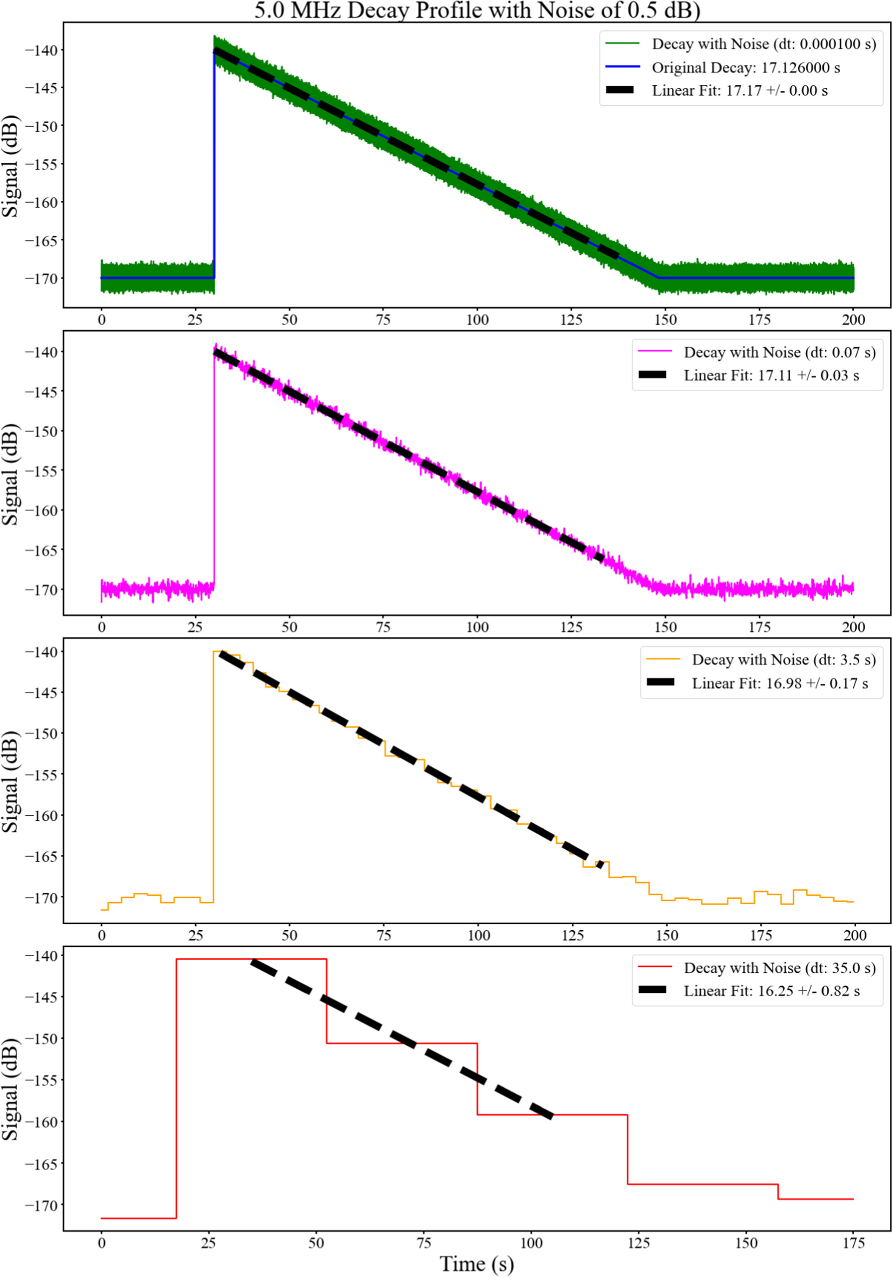
Figure B1. Synthetic light curves at 5 MHz derived as a power-law function between the maximum and the background values from Figure 4 of V. Krupar et al. (2020) with a random noise with a 0.5 dB standard deviation superimposed. The black dashed line corresponds to a power-law fit on these data.
Download figure: