ALMA Observations of Io Going into and Coming out of Eclipse (original) (raw)
Jupiter’s satellite Io is unique among bodies in our solar system. Its yellow–white–orange–red coloration is produced by SO2 frost on its surface, a variety of sulfur allotropes (S2–S20), and metastable polymorphs of elemental sulfur mixed in with other species (Moses & Nash 1991). Spectra of the numerous dark calderas, sites of intermittent volcanic activity, indicate the presence of (ultra)mafic minerals such as olivine and pyroxene (Geissler et al. 1999). When Io is in eclipse (Jupiter’s shadow), or during an Ionian night (visible only from spacecraft), visible and near-infrared images of the satellite reveal dozens of thermally bright volcanic hot spots (e.g., Geissler et al. 2001; Macintosh et al. 2003; de Pater et al. 2004; Spencer et al. 2007; Retherford et al. 2007). This widespread volcanic activity is powered by strong tidal heating induced by Io’s orbital eccentricity, which is the result of the Laplace orbital resonance between Io, Europa, and Ganymede. Some volcanoes are associated with active plumes, which are a major source of material into Io’s atmosphere, Jupiter’s magnetosphere, and even the interplanetary medium. The mass loss from Io’s atmosphere is estimated at 1 ton s−1 (Spencer & Schneider 1996), yet the atmosphere is consistently present, indicating an ongoing replenishment mechanism. However, the amount of material pumped into Io’s atmosphere by volcanism is not well known, and it is consequently not known whether the dynamics in Io’s atmosphere is primarily driven by sublimation of SO2 frost on its surface or by volcanoes. An additional source of atmospheric gas may be sputtering from Io’s surface.
A decade after the initial detection of gaseous SO2 in its _ν_3 band (7.3 _μ_m) from Voyager data (Pearl et al. 1979), Io’s “global” SO2 atmosphere was detected at 222 GHz (Lellouch et al. 1990). These data revealed a surface pressure of order 4–40 nbars (2 × 10¹⁷–2 × 1018 cm−2), covering 3%–20% of the surface, at temperatures of ∼500–600 K. There is a large uncertainty in the temperature, however, as it is extremely difficult to disentangle the contributions of density, temperature and fractional coverage8 in the line profiles (e.g., Lellouch et al. 1992). Moreover, zonal winds would broaden the line profile (“competing” with temperature), while Ballester et al. (1994) noted that winds from volcanic eruptions may distort the line shape, both adding complications to modeling efforts. Although SO2 has now been observed at millimeter, UV, and at thermal infrared wavelengths, its temperature and column density are still poorly constrained.
Based upon photochemical considerations alone, in a SO2-dominated atmosphere, one would expect at least the products SO, O2, as well as atomic S and O (e.g., Kumar 1985; Summers 1985). SO was detected at millimeter wavelengths at a level of a few percent compared to the SO2 abundance (Lellouch 1996). While O2 has not (yet) been detected, S and O have been detected, e.g., in the form of auroral emissions off Io’s limb along its equator (e.g., Geissler et al. 2004b). We further note that gaseous NaCl was first detected by Lellouch et al. (2003), and a tentative detection of KCl was reported by Moullet et al. (2013). Both NaCl and KCl were mapped with ALMA by Moullet (2015).
Spatially resolved data obtained with the Hubble Space Telescope (HST) at UV wavelengths revealed that SO2 was mainly confined to latitudes within 30°–40° from the equator, with a higher column density and latitudinal extent on the anti-Jovian side (central meridian longitude CML ∼ 180°W; e.g., Roesler et al. 1999; Feaga et al. 2009). The sub-(CML ∼0°W) to anti-Jovian hemisphere distribution was confirmed using disk-averaged thermal infrared data of the 19 _μ_m _ν_2 band of SO2, observed in absorption against Io with the TEXES instrument on NASA’s Infrared Telescope Facility (IRTF) in 2001–2005 (Spencer et al. 2005). While these observations showed a temperature of ∼115–120 K, interpretation of disk-resolved observations of the SO2 _ν_1 + _ν_3 band at 4 _μ_m with the CRIRES instrument on the Very Large Telescope (VLT) favors a temperature of ∼170 K (Lellouch et al. 2015). Typical column densities in all these data vary roughly from ∼1016 on the sub-Jovian hemisphere to ∼1017 cm−2 on the anti-Jovian side.
Moullet et al. (2010) used the spatial distribution derived from the HST/UV and TEXES/IRTF observations to analyze SO2 maps at millimeter wavelengths obtained with the Sub-Millimeter Array (SMA). By decreasing the number of free parameters to just temperature and column density, using the fractional coverage from the UV and mid-IR data, they derived a disk-averaged column density of 2.3–4.6 × 1016 cm−2 and temperature between 150–210 K on the leading (CML ∼ 90°W) hemisphere, and 0.7–1.1 × 1016 cm−2 with 215–255 K on the trailing (CML ∼ 270°W) side. These temperatures and column densities are considerably lower than the earlier millimeter-wavelength measurements.
As mentioned above, it is still being debated whether the primary source of Io’s atmosphere is volcanic or driven by sublimation, although it is clear that both volcanoes and SO2 frost do play a role (Lellouch et al. 1990, 2003, 2015; Spencer et al. 2005; Jessup et al. 2007; Moullet et al. 2010, 2013; Tsang et al. 2012, 2016; Moullet 2015). Although much of the SO2 frost may ultimately have been produced by volcanoes, the extent to which volcanoes directly affect the atmosphere is unknown; moreover, this likely varies over time. Mid-IR observations showed an increase in SO2 abundance with decreasing heliocentric distance, which is, at least in part, in support of the sublimation theory (Tsang et al. 2012). Further support was given by the analysis of the SMA maps mentioned above, which indicated that frost sublimation is the main source of gaseous SO2, and photolysis of SO2 is the main source of SO, because volcanic activity is not sufficient to explain the SO column density and distribution (Moullet et al. 2010). On the other hand, SO2 gas is enhanced above some volcanic hot spots (McGrath et al. 2000), and Pele’s plume contains the sulfur-rich gases S2, S, and SO (McGrath et al. 2000; Spencer et al. 2000; Jessup et al. 2007), indicative of volcanic contributions to Io’s atmosphere. For more information on the pros and cons of the driving forces (sublimation versus volcanic) of Io’s atmospheric dynamics, see the excellent reviews of the state of knowledge of Io’s atmosphere in the mid-2000s by McGrath et al. (2004) and Lellouch et al. (2007).
Observations of Io right before, after, and during an eclipse provide the best way to separate the volcanic from sublimation-driven contributions to its atmosphere. The atmospheric temperature is expected to drop within minutes after Io enters an eclipse (e.g., de Pater et al. 2002). The SO2 gas that makes up the bulk of Io’s atmosphere is expected to condense out on a similar timescale, set by the vapor pressure of this gas, which is a steep exponential function of temperature (_P_vapor = 1.52 × 10⁸_e_−4510/T bar; Wagman 1979).
Tsang et al. (2016) obtained the first direct observations of the SO2 _ν_2 band in Io’s atmosphere in eclipse with the TEXES instrument on the Gemini telescope. Their disk-integrated spectra were sensitive to surface temperature, atmospheric temperature, and SO2 column abundance. Based on a simple model with a surface temperature of 127 K, they found that this value dropped to 105 K within minutes after entering eclipse. A range of models for Io’s atmospheric cooling all showed that the SO2 column density simultaneously dropped, by a factor of 5 ± 2. They, therefore, concluded that the atmosphere must contain a large component that is driven by sublimation.
Although the radical SO will not condense at these temperatures, it may be rapidly removed from the atmosphere through reactions with Io’s surface (Lellouch 1996). However, a bright emission band complex at 1.707 _μ_m, the forbidden electronic transition of SO, was observed in a disk-integrated spectrum of Io while in eclipse. Based on the line width, a rotational temperature of ∼1000 K was derived, and the authors concluded that excited SO molecules were ejected from the then very active volcano Loki Patera (de Pater et al. 2002).
More recent observations reveal the spatial distribution of SO and show that the correlation with volcanoes is tenuous at best (de Pater et al. 2007, 2020). Both the spatial distribution and the spectral shape of the SO emission band vary considerably across Io and over time. In their most recent paper (de Pater et al. 2020), the authors suggest that the emissions are likely caused by a large number of stealth plumes, “high-entropy” eruptions (Johnson et al. 1995) produced through the interaction of silicate melts with superheated SO2 vapor at depth. These plumes do not have much dust or condensates and are therefore not seen in reflected sunlight. The SO data are further suggestive of non-LTE processes, in addition to the direct ejection of excited SO from the volcanic vents.
In order to shed more light on the core question whether the dynamics in Io’s atmosphere is predominantly driven by sublimation of SO2 ice or volcanic activity, we present spatially resolved observations of the satellite at 880 _μ_m when Io moved from sunlight into eclipse, and half a year later from eclipse into sunlight. The observations and data reduction are discussed in Section 2 with results presented in Section 3. The analysis of line profiles is presented in Section 4, with a discussion in Section 5. Conclusions are summarized in Section 6.
We observed Io with the Atacama Large (sub)Millimeter Array (ALMA) on 2018 March 20 just before and after the satellite moved into eclipse. Similar experiments were conducted when Io moved out of eclipse on 2018 September 2 and 11. Figure 1 shows the viewing geometry on both occasions. All observations were conducted in Band 7, the 1 mm band. Each continuous observation of a source (calibrator or Io) is referred to as a scan and gets a scan “label.” Amplitude and bandpass calibrations were performed on the radio source J1517–2422 during the first ∼15 minutes of each of the six ∼35 minute long observing sessions (two sessions on each date). The phases were calibrated on J1532–1319 in March and on J1507–1652 in September. These observations or scans (typically 30–60 s long) were taken before, interspersed between, and at the end of the Io observations. Typical Io scans are 6–7 minutes long, though toward the end of the observing sessions, they usually lasted for only 1–2 minutes. The flux densities of J1517–2422 were checked with the ALMA calibrator catalog; no updates have been needed since the observatory’s initial pipeline data reduction. On September 11, the flux densities of both Io and the secondary calibrator were much lower for the in-eclipse data than for the ones in sunlight, perhaps caused by some decorrelation in the phases and/or pointing errors. We therefore multiplied the Io-in-eclipse data by a factor of 1.15, the ratio for the secondary calibrator between the in-sunlight and in-eclipse data sets.
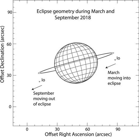
Figure 1. Geometries of Io moving into eclipse (2018 March) and coming out of eclipse (2018 September). (Adapted from the Planetary Ring Node: http://pds-rings.seti.org/tools/).
Download figure:
Standard imageHigh-resolution image
We observed several transitions of SO2 and SO, and one transition of KCl. These transitions, together with the spectral window (spw) used to observe them, the total bandwidth, and channel width of each spw, are listed in Table 1. We typically had three to four beams (resolution elements) across the satellite. Usually, all scans on a particular source are combined to create a map or a spectral-line data cube. Because we are interested in particular in how the spatial brightness distribution and flux density change during eclipse ingress and egress, we imaged individual scans, and even fractions of a scan, as summarized in Table 2.
**Table 1.**ALMA Data: Species and Frequencies
| Species | Frequency | Wavelength | Line Strength | E (low) | Spectral Window | Bandwidth | Channel Width |
|---|---|---|---|---|---|---|---|
| (GHz) | mm | (cm−1 mol−1 cm−2) | (cm−1) | spw | Total (MHz) | (kHz) | |
| Continuum | 334.100 | 0.897 | 0 | 2000 | 15625 | ||
| SO2 | 346.524 | 0.865 | 6.18556E-22 | 102.750 | 1 | 117 | 122 |
| SO | 346.528 | 0.865 | 5.34047e-21 | 43.1928 | 1 | 117 | 122 |
| SO2 | 346.652 | 0.865 | 1.11142E-21 | 105.299 | 2 | 117 | 122 |
| SO | 344.311 | 0.871 | 4.50069e-21 | 49.3181 | 3 | 117 | 122 |
| KCl | 344.820 | 0.869 | 2.23552e-19 | 253.489 | 4 | 117 | 122 |
| SO2 | 332.091 | 0.903 | 3.10870e-22 | 141.501 | 5 | 117 | 122 |
| SO2 | 332.505 | 0.902 | 2.65693e-22 | 10.6590 | 6 | 58.6 | 122 |
| SO2 | 333.043 | 0.900 | 2.42761e-23 | 643.771 | 7 | 58.6 | 122 |
Note. All transitions are taken from https://spec.jpl.nasa.gov.
Download table as: ASCIITypeset image
**Table 2.**Time Table of Observations in 2018
| Date Start time | End Time | Sub-long. | Sub-lat. | Scans | Diameter Io | Array conf. | HPBW | HPBW | Comments |
|---|---|---|---|---|---|---|---|---|---|
| (month-day hr:m:s) | (hr:m:s) | (deg (W)) | (deg) | (combined) | (arcsec) | (arcsec) | (km) | ||
| 03-20 10:02:29 | 10:21:41 | 337.2 | −3.40 | 7, 11, 15 in set 1 | 1.058 | C43-4 | 0.35 | 1205 | sunlight |
| 03-20 10:54:43 | 11:01:18 | 343.7 | −3.40 | 7 in set 2 | 1.058 | C43-4 | 0.35 | 1205 | eclipse |
| 03-20 10:54:43 | 10:57:40 | 343.4 | −3.40 | 7a in set 2 | 1.058 | C43-4 | 0.35 | 1205 | eclipse |
| 03-20 10:57:40 | 11:01:18 | 343.8 | −3.40 | 7b in set 2 | 1.058 | C43-4 | 0.35 | 1205 | eclipse |
| 03-20 11:03:19 | 11:13:54 | 345.1 | −3.40 | 11, 15 in set 2 | 1.058 | C43-4 | 0.35 | 1205 | eclipse |
| 09-02 21:46:21 | 21:53:00 | 19.5 | −2.96 | 6 in set 1 | 0.885 | C43-3 | 0.30 | 1235 | (partial) eclipse |
| 09-02 21:46:21 | 21:49:40 | 19.2 | −2.96 | 6a in set 1 | 0.885 | C43-3 | 0.30 | 1235 | eclipse |
| 09-02 21:49:40 | 21:53:00 | 19.7 | −2.96 | 6b in set 1 | 0.885 | C43-3 | 0.30 | 1235 | partial eclipse |
| 09-02 21:54:01 | 22:00:36 | 20.5 | −2.96 | 8 in set 1 | 0.885 | C43-3 | 0.30 | 1235 | sunlight |
| 09-02 21:54:01 | 21:57:20 | 20.3 | −2.96 | 8a in set 1 | 0.885 | C43-3 | 0.30 | 1235 | sunlight |
| 09-02 21:57:20 | 22:00:36 | 20.7 | −2.96 | 8b in set 1 | 0.885 | C43-3 | 0.30 | 1235 | sunlight |
| 09-02 22:01:22 | 22:04:28 | 21.3 | −2.96 | 10, 12 in set 1 | 0.885 | C43-3 | 0.30 | 1235 | sunlight |
| 09-02 22:22:00 | 22:40:08 | 25.3 | −2.96 | 6, 8, 10, 12 in set 2 | 0.885 | C43-3 | 0.30 | 1235 | sunlight |
| 09-11 17:36:12 | 17:54:03 | 14.8 | −2.95 | 6, 8, 10, 12 in set 1 | 0.867 | C43-5 | 0.22 | 924 | eclipse |
| 09-11 18:24:01 | 18:41:56 | 21.5 | −2.95 | 6, 8, 10, 12 in set 2 | 0.867 | C43-5 | 0.22 | 924 | sunlight |
Note. Io’s diameter is 3642 km. Sub-long, sub-lat are Observers’ sub-longitude and sub-latitude. On each day, two sets of data were taken, typically one when Io was in eclipse and one when it was in sunlight. Scans 6, 7, 8, and 11 are 6–7 minutes long; scans 10, 12, and 15 are typically 1–2 minutes long.
March 20: partial eclipse started at 10:46:40; full eclipse started at 10:50:22.
September 2: partial eclipse started 21:49:45 and ended 21:53:29.
September 11: partial eclipse started 18:13:52 and ended: 18:17:35. There was no difference between sunlight scans 6, 8, 10, and 12, nor between the first and last half of sunlight scan 6.
Download table as: ASCIITypeset image
After the calibration and initial flagging was done in the ALMA pipeline, we split off the Io data into its own data set (referred to as a measurement set, Io.ms) and attached a new ephemeris file so that the position and velocity got updated every minute of time. We used the Common Astronomy Software Applications package, CASA, version 5.4.0-68 for all our data reduction. This version properly handles the tracking of Io’s motion across the sky and velocity along the line of sight. Our final products are centered on Io, both in space (images) and velocity (line profiles). We first created continuum maps of the satellite, used initially for additional flagging and self-calibration of the data (e.g., Cornwell & Fomalont 1999). Mapping was done using tCLEAN; a model of Io’s continuum emission served as a “startmodel” in the deconvolution (“cleaning”) and self-calibration process. The model is a uniform limb-darkened disk with a disk-averaged brightness temperature that matches the data (typically between 65 and 80 K) and a limb-darkening coefficient q = 0.3 (i.e., the brightness falls off toward the limb as cos θ q, with θ the emission angle). All data were self-calibrated twice (phase selfcal only), although the second self-calibration did not improve the data substantially over the first one.
Before creating spectral-line data cubes, we split out each spectral window (Table 1) into its own measurement set (Io-spwx.ms, with x = 0–7) and subtracted the continuum emission from each Io-spwx.ms (x = 1–7) data set using the CASA routine UVCONTSUB. At this point, we have spectral image data cubes of just the emission of each species (SO2, SO, KCl).
In order to create maps of the brightness distribution of each species at a high signal-to-noise ratio (S/N), we averaged the data in velocity over 0.4 km s−1, centered at the center of each line; these maps are referred to as “line center maps.” To evaluate line profiles, we also constructed three-dimensional (3D) data cubes with R.A. and decl. along the _x_- and _y_-axes, and frequency (or velocity) along the _z_-axis, where each image plane was averaged over 0.142 km s−1, which translates roughly into a frequency resolution of ∼160 kHz,9 slightly larger than the 122 kHz width of an individual channel in each spw. All (spectral line, line center, and continuum) maps were constructed using uniform weighting and cleaned using the Clark or Högbom algorithm with a gain of 10% in CASA’s tCLEAN routine. In essence, in this routine, we iteratively remove 10% of the peak flux density from that location on the map, together with the synthesized beam (the telescope’s antenna pattern). This process is repeated until essentially only noise is left in the “residual” map. These so-called “clean components” form a map, the .model map in CASA. An example is shown in Figure 2. (Note that the continuum maps were deconvolved using a startmodel in tCLEAN, as described above). The .model map is convolved with a circular Gaussian beam with a full width at half power (HPBW) that best matches the inner part of the synthesized beam (see Table 2 for the HPBW values) before being added back to the residual map. The .model map in Figure 2 shows the clean components of the map displayed in the top-left panel in Figure 4, discussed below in Section 3.2. We used a cell (or pixel) size for all maps of 0 04, i.e., between 5.5 and 9 pixels/beam.
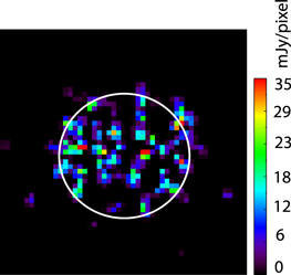
Figure 2. This model map shows the sum of all CLEAN components per pixel as obtained from CASA’s tCLEAN routine when deconvolving the original Io-in-sunlight map at 346.652 GHz. After convolution with the HPBW and restoration to the residual map, this particular .model map results in the map displayed in the top-left panel of Figure 4.
Download figure:
Standard imageHigh-resolution image
3.1. Continuum Maps
The continuum maps for each of the six sessions, three in sunlight and three in eclipse, are very similar and do not show any structure other than that the maximum temperature is not centered on Io, but slightly displaced toward the afternoon, as shown in Figures 3(a) and (b). We determined the total flux density from such maps, because it is impossible to determine this from the uv data, as these are dominated by the signal from nearby Jupiter. For the maps in eclipse, the sidelobe patterns from Jupiter produce broad (similar size as Io) low-level (few percent of Io’s peak intensity) negative and/or positive ripples which affect the precise determination of Io’s flux density. Although ideally one would subtract Jupiter from the visibility data, in practice this is not easy as Jupiter is not a uniform disk at millimeter wavelengths (e.g., de Pater et al. 2019), moves with respect to Io, is mostly resolved out, and mostly on the edge or outside the ∼20″ primary beam. We therefore opted to correct for these negative or positive backgrounds by subtracting the average flux density per pixel as determined from an annulus around Io in each of the six maps. Each map was constructed from all scans in the particular observing session, although the in-eclipse scan from 6 on September 11 was not used (too affected by nearby Jupiter).
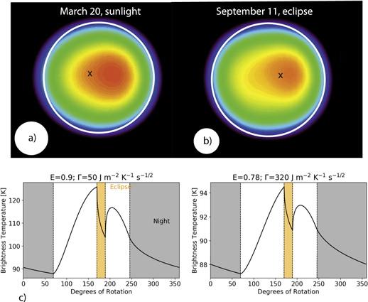
Figure 3. Continuum image of Io at 334.1 GHz taken on 2018 March 20 while Io was in sunlight (panel a) and on September 11 while Io was in eclipse (panel b). Io north is up in these images. The white circle shows the approximate size of Io’s disk. The X indicates the approximate subsolar location, and the approximate beam size is indicated in the lower-left corner. The temperature scale is from 0 to ∼90 K, but not quite linear to bring out the slight asymmetry in the emission. (c) Simple thermal conduction model at midlatitudes that can explain the differences in brightness temperature between the infrared and millimeter data when entering an eclipse. (See text for details).
Download figure:
Standard imageHigh-resolution image
The total flux density, F J, normalized to a geocentric distance of 5.044 au (Io’s diameter is 1″ at this distance) and averaged over all six measurements, F J = 5.43 ± 0.15 Jy, which translates into a disk-averaged brightness temperature, T b = 93.6 ± 2.5 K. Because Io blocks the cosmic microwave background radiation (CMB), which is 0.044 K at this wavelength, we have added this value to all brightness temperatures quoted. The uncertainties quoted above are the standard deviation or rms spread in the continuum measurements, which is much larger than the uncertainty in any single continuum measurement based on the rms in the maps, which varies from 0.001–0.008 Jy (0.02–0.14 K) in sunlight, to 0.008–0.05 Jy (0.14–0.86 K) in eclipse. For absolute values, we need to add the calibration uncertainty in quadrature. A typical calibration error for ALMA data is ∼5%, i.e., the total uncertainty on the brightness temperature is ∼5 K.
For all three dates, there is a small difference between T b in sunlight and in eclipse: in sunlight, we find F = 5.43 ± 0.11 Jy (5.43, 5.39, 5.59 Jy, in chronological order), i.e., T b = 93.6 ± 1.8 K, and in eclipse F = 5.25 ± 0.14 Jy (5.16, 5.25, 5.44 Jy), i.e., T b = 90.8 ± 2.2 K. The uncertainties are again the rms spread in the data points. The difference between these numbers, and because all in-eclipse values are lower than the corresponding in-sunlight values, suggests that T b may decrease by ∼3 K after entering eclipse. This is interesting because at mid-IR wavelengths, Io’s surface temperature dropped steeply within minutes after entering eclipse (Morrison & Cruikshank 1973; Sinton & Kaminsky 1988). Tsang et al. (2016) measured a drop in surface temperature at 19 _μ_m from 127 to 105 K. At radio wavelengths we typically probe ∼10–20 wavelengths deep into the crust, or ∼1–2 cm at the ALMA wavelengths used (for pure ice, this can be hundreds of wavelengths deep). Hence, even after having been in shadow for ∼2 hr, the temperature at depth had decreased by no more than ∼3 K.
The morning–afternoon asymmetry in Io’s continuum brightness is also still present during eclipse, or after having been in darkness for ∼2 hr (Figure 3(b)), which further supports our finding that eclipse cooling at depth is slow. We used a simple thermal conduction model (after the infrared version of the de Kleer et al. (2020) model), ignoring albedo variations across Io’s surface (which may be reasonable given our relatively low spatial resolution), to demonstrate that the difference between the eclipse cooling at infrared and millimeter wavelengths can be explained if the upper ∼cm or so of Io’s crust is composed of two layers. For the model in Figure 2(c), we assumed a bolometric Bond albedo, A = 0.5, an infrared emissivity  = 0.9, and a thermal inertia Γ = 50 J m−2 K−1 s−1/2. This number is similar to the value of 70 J m−2 K−1 s−1/2 derived by Rathbun et al. (2004) from Galileo/PPR data. At millimeter wavelengths, we assumed A = 0.5, = 0.78, and Γ = 320 J m−2 K−1 s−1/2. These models, for a “typical” surface location at midlatitudes, more or less match the data and suggest that Io’s surface is overlain with a thin (no more than a few millimeters thick) low-thermal-inertia layer, such as expected for dust or fluffy deposits from volcanic plumes, overlying a more compact high-thermal-inertia layer, composed of ice (likely coarse grained and/or sintered) and rock. This is very similar to the model proposed by Morrison & Cruikshank (1973) based upon seven eclipse ingress or egress measurements at a wavelength of 20 _μ_m, although our value for the low-thermal-inertia layer is ∼4 times higher. Sinton & Kaminsky (1988) analyzed 13 observations of eclipse ingress and egress in the early 1980s at wavelengths between 3.5 and 30 _μ_m. They found a best fit by assuming Io to be covered by both dark (A = 0.10) and bright (A = 0.47) areas, with Γ = 5.6 and 50 J m−2 K−1 s−1/2, respectively, where the low-thermal-inertia layer is just a thin layer atop a much higher thermal inertia. They noted that cooling was rapid during the first few minutes, followed by a slower process that they attributed to a combination of the higher thermal inertia, higher albedo passive component, and emission from hot spots. Although their thermal inertias are roughly an order of magnitude smaller than the values we found, the overall physical picture of a thin dusty/porous layer atop a more compact high-inertia layer is the same for all models. Our millimeter data in particular add a strong constraint to the higher-thermal-inertia layer roughly a centimeter or so below Io’s surface, a depth not probed at shorter wavelengths. Our values for the upper dusty layer are also similar to those reported for the other Galilean satellites (e.g., Spencer 1987; Spencer et al. 1999; de Kleer et al. 2020), and they agree with the best-fit values found in the thermophysical parametric study by Walker et al. (2012). Note, though, that the latter study, as well as other two-component thermal inertia studies at mid-IR wavelengths, all refer to horizontal surface variations, while our study refers to a vertically stacked model. In a future paper, we intend to expand our two-layer model to include proper dark and bright surface areas, as done for Ganymede in de Kleer et al. (2020).
3.2. Line Center Maps (Averaged over 0.4 km s−1)
3.2.1. Line Center Maps on 2018 March 20
SO 2 _maps_—Figure 4 (top row) shows SO2 maps at 346.652 GHz (spw2), averaged in velocity over 0.4 km s−1 (∼0.45 MHz) centered on the line, from 2018 March 20 when Io went into eclipse. The bottom row shows simultaneously taken SO maps (averaged over both transitions to increase the S/N). The first panel shows Io in sunlight, and the next two panels show the satellite ∼6 and ∼15 minutes after entering eclipse (Table 2). The large circle shows the outline of Io, as determined from simultaneously obtained images of the continuum emission. As soon as Io enters an eclipse, the atmospheric and surface temperatures drop (Figure 3), and SO2 is expected to condense out on a timescale t ∼ H/c s ≈ 70 s, for a scale height H ≈ 10 km and sound speed c s ≈1.5 × 104 cm s−1 (de Pater et al. 2002), unless a layer of noncondensible gases prevents complete collapse (Moore et al. 2009). Once in eclipse, assuming complete collapse, the only SO2 we see should be volcanically sourced. The letters on Figure 4 show the positions of Karei Patera (K), Daedalus Patera (D), and North Lerna (L). Due to the excellent match between the location of these volcanoes and the SO2 emissions on this day, these volcanoes are likely the main sources of SO2 gas for Io in eclipse. All three volcanoes have shown either plumes or changes on the surface attributed to plume activity in the past (Geissler et al. 2004a; Spencer et al. 2007).
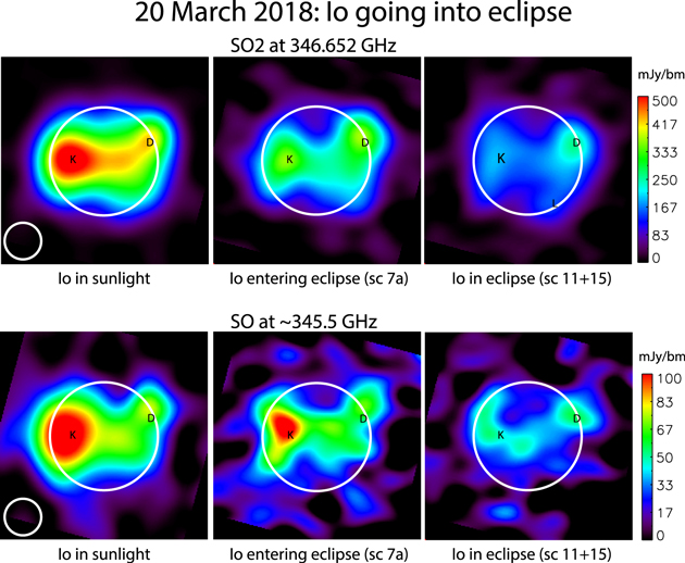
Figure 4. Top row: maps of the spw2 data of the SO2 distribution on Io in sunlight, and ∼6 (scan 7a) and ∼15 (scans 11+15) minutes after entering eclipse. Bottom row: maps of the averaged spw1 and spw3 SO data taken at the same times as the SO2 maps. All maps were averaged over 0.4 km s−1 (∼0.45 MHz). Io north is up in all frames. The large circle shows the outline of Io, and the small circle in the lower left shows the size of the beam (HPBW). The volcanoes Karei Patera (K), Daedalus Patera (D), and North Lerna (L, on one panel only) are indicated.
Download figure:
Standard imageHigh-resolution image
_SO maps_—SO can be volcanically sourced, i.e., produced in thermochemical equilibrium in the vent (Zolotov & Fegley 1998), or later via the reaction O + S2 at a column-integrated rate of 4.6 × 1011 cm−2 s−1, or while in sunlight it can be produced through photolysis of SO2 at a similar column-integrated rate (Moses et al. 2002). About 70% of SO is lost through photolysis into S and O, but during an eclipse, the only known loss is through a reaction with itself: 2SO SO2 + S, at a rate of 3.25 × 1010 cm−2 s−1 (Moses et al. 2002). Hence, to eliminate an entire column of 1015 cm−2 (Section 4.3) would take 8.5 hr, or almost an hour to lose a 10× smaller column. Hence, one would not expect much change in the SO column density upon eclipse ingress. The data, however, clearly show a decrease in the SO emission after eclipse ingress, though not as fast as for SO2. The observed decrease suggests that SO may be much more reactive with itself than captured by the above reaction rate. Additional (in-between) reactions are 2SO (SO)2, and SO + (SO)2 S2O + SO2 (Schenk & Steudel 1965). At low temperatures (i.e., in eclipse), both SO2 and S2O condense out, and hence SO may effectively condense out through chemical reactions in the gas phase with the surface, producing the above-mentioned compounds (Hapke & Graham 1989). Based on our observations, it looks like such self-reactions of SO must be very fast. Although this possibility has been suggested in the past (e.g., Lellouch 1996), the SO “condensation” rate has never before been observed.
As shown, the connection with volcanoes is more tenuous for the SO emissions than for SO2, except perhaps for Daedalus Patera. However, as noted above, SO’s column density is not really expected to change much. With a layer of SO, and perhaps other noncondensible species (e.g., O, O2), SO2 may indeed not completely collapse, such as modeled b,y e.g., Moore et al. (2009). We may also see emissions from stealth volcanoes, as postulated by de Pater et al. (2020) to explain the widespread spatial distribution of the 1.707 _μ_m SO emissions, which only occasionally showed a connection to volcanoes.
_Disk-integrated flux densities_—We integrated the flux density over Io on each map for each transition (except spw7, the lowest line strength, where we have no detection), and plotted the results on the left panel of Figure 5. For easier comparison, all flux densities in this figure have been normalized to a geocentric distance of 5.044 au, at which distance Io’s diameter is 1″. Assuming that Io’s flux density is constant while in sunlight, it decreases exponentially within the first few minutes after the satellite enters eclipse. The dotted lines show the collapse for each transition, modeled for the SO2 lines as
where F i stands for the flux density in each transition i (for i = spw1, spw2, spw5, and spw6), t j the time (in minutes) from time _t_0 = 0 taken as midway during the partial eclipse, _t_1 = 8, _t_2 = 10.7, _t_3 = 19.5 minutes). H i shows the exponential decay constant in minutes (indicated on the figure). After the initial drop in intensity, further decrease is slowed down, as roughly indicated by the term C i(t j − _t_1), with C = 1 at 346.524 and 332.091 GHz (spw1, spw5), C = 0.6 at 346.652 GHz (spw2), and C = 0.7 at 332.505 GHz (spw6). A new “steady state” appears to be reached within ∼20 minutes, similar to the results shown by Tsang et al. (2016) at 19 _μ_m. The flux density decreases by a factor of 2 at 346.524, 332.091, and 332.505 GHz (spw1, spw5, spw6), and by 3.2 at the strongest line transition, 346.652 GHz (spw2). As shown by H i, the latter flux density decreases much faster than the others. Also, the SO emission, plotted here as the average of the two transitions, decreases by a factor of 2, although much more gradual, essentially following a linear decay, modeled as
where a = −15 mJy minute−1. This more gradual decrease is also visible on the maps in Figure 4.
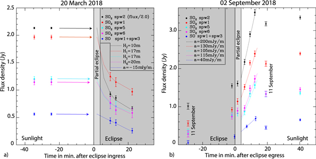
Figure 5. Flux densities integrated over individual maps (as in Figures 4, 6, and 7) as a function of time (filled circles for March 20 and September 2; crosses (x) for September 11). The colors refer to different spectral windows. The data for SO were averaged over spw1 and spw3 to increase the S/N. The dotted lines superposed on the data in panel (a) show the exponential decrease (Equation 1) or the linear slope (Equation 2) after entering eclipse, whichever is appropriate. In panel (b), the dotted lines show the linear increase after emerging from eclipse on September 2. All data are normalized to a geocentric distance of 5.044 au.
Download figure:
Standard imageHigh-resolution image
3.2.2. Line Center Maps on 2018 September 2 and 11
2018 September 2—Figure 6 shows the distribution of SO2 and SO gases on 2018 September 2, when Io moved from eclipse into sunlight. The integrated flux densities are plotted on the right-side panel in Figure 5. As soon as sunlight hits the satellite, SO2 starts to sublime and within 10 minutes the atmosphere has re-formed in a linear fashion. The flux density in each transition increased by roughly a factor of 2. SO increased by roughly a factor of 3, also in a linear fashion. The dotted lines on the figure were calculated using Equation (2); the values for a in mJy minute−1 (positive sign for increasing slope) are indicated on the figure.
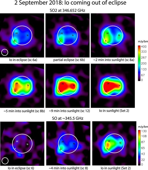
Figure 6. Top two rows: maps of the spw2 data of the SO2 distribution on Io in eclipse (scan 6a), and emerging into sunlight on 2018 September 2, starting with a partial eclipse (scan 6b), as indicated. Bottom row: maps of the averaged spw1 and spw3 SO data. All maps were averaged over 0.4 km s−1 (∼0.45 MHz). See Table 2 for exact times of each scan. Io north is up. The large circle shows the outline of Io. The small circle in the lower left shows the HPBW. The letters show the positions of several volcanoes: P for P207, Pf for PFd1691, and N for Nyambe Patera.
Download figure:
Standard imageHigh-resolution image
When the satellite was in eclipse on September 2 (scan 6a in Figure 6 ), the spatial distribution of SO2 gas shows very strong emission near the SW limb, centered on P207 (910W long., 370S lat.), a small dark-floored patera. Although thermal emission has been detected at this site with the W. M. Keck Observatory (Marchis et al. 2005; de Kleer & de Pater 2016), no evidence of plume activity has ever before been recorded. Faint emissions can further been seen near Nyambe Patera and just north of PFd1691, a dark-floored patera where thermal emission has also been detected with the Keck Observatory (de Kleer et al. 2019). As soon as Io enters sunlight (scan 6b), the SO2 emission near P207 becomes more pronounced; this is the side of Io where the Sun first strikes. Over the next 4–5 minutes (scans 8a, 8b), the emissions get stronger, in particular near the volcanoes. At 9 minutes (scan 12), the SO2 atmosphere has completely re-formed.
The bottom row in Figure 6 shows practically no SO emissions while Io is in eclipse (scan 6), except for some emission along the limb north and south of P207. Faint emissions are also seen near PFd1691 and at a few other places on the disk. None of these emissions seem to be directly associated with known volcanoes nor with the SO2 emissions on Io in eclipse. About 4 minutes after entering sunlight (scan 8), strong SO emission is detected above P207, suggestive of formation through photodissociation of SO2. Five minutes later, we also detect emissions over Nyambe Patera, and another 20–30 minutes later, the SO emissions track the SO2 emissions pretty well, as expected if the main source of SO is photolysis of SO2.
2018 September 11—Figure 7 shows the spatial distributions of SO2 and SO of Io in eclipse and in sunlight on 2018 September 11, but not during the transition from eclipse into sunlight. While in eclipse, faint volcanically sourced SO2 emissions are present near P129, Karei, and Ra Paterae, and along the west limb near Gish Bar Patera and NW of P207. The eruption at P207, so prominent 9 days earlier, has stopped. No SO emissions are seen above the noise level. Ten minutes later, the atmosphere has re-formed as shown by the in-sunlight map, with most of the emissions confined to latitudes within , in agreement with the latitudinal extent measured from UV/HST data (Feaga et al. 2009) and with Figures 4 and 6. The SO map shows emission peaks above Karei Patera and P129. The ratio of flux densities between Io in sunlight and in eclipse is about a factor of 4–5 for SO2 and ∼10 for SO on this day (Figure 5). Hence, as shown by both this large ratio and the maps, on this date, there was not much volcanic activity.
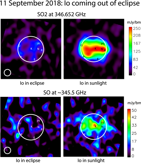
Figure 7. Top row: maps of the spw2 data of the SO2 distribution on Io in eclipse and in sunlight on 2018 September 11. Bottom row: maps of the SO distribution on Io in sunlight and in eclipse on 2018 September 11. The maps from spw1 and spw3 were averaged to increase the S/N. Io north is up in these frames. All maps were averaged over 0.4 km s−1 (∼0.45 MHz). The large circle shows the outline of Io. The small circle in the lower left shows the HPBW. Note that the beam is smaller than in Figures 6 and 4, so that the intensity scale on the right shows values that are much smaller than in the other figures. The letters show the positions of several volcanoes: P: P207; G: Gish Bar Patera; K: Karei Patera; N: Nyambe Patera; P1: P129; R: Ra Patera; E: Euboea.
Download figure:
Standard imageHigh-resolution image
3.2.3. Map of KCl on 2018 March 20
On 2018 March 20, we also detected KCl, shown in Figure 8. As shown, the distribution is completely different from that seen in SO2 and SO: the southeastern spot is centered near Ulgen Patera, and emission is seen along the limb toward the north. There may also be some emission from near Dazhbog Patera. KCl was not detected in 2018 September, when Ulgen Patera was out of view. Further analysis of the KCl data will be provided in a future paper.
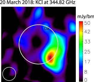
Figure 8. Map of the spatial distribution of KCl on 2018 March 20. The map was averaged over 0.4 km s−1 (∼0.45 MHz). Io north is up in this frame. This map is from the sunlight data only and is essentially the same as one in which sunlight and eclipse data are averaged. The volcanoes indicated on this map are U: Ulgen Patera; Da: Dazhbog Patera.
Download figure:
Standard imageHigh-resolution image
3.3. SO2 Line Profiles and Image Data Cubes (Resolution 0.142 km s−1 ≈ 160 kHz)
In addition to the spatial distribution at the peak of the line profiles (i.e., the line center maps) when Io goes from sunlight into eclipse and vice versa, the full image data cubes contain an additional wealth of information.
3.3.1. Image Data Cubes on 2018 March 20
In Figure 9, we show several frames of the SO2 image data cubes together with disk-integrated line profiles from 2018 March 20 for Io in sunlight (top half) and in eclipse (bottom half). To increase the S/N, we averaged the data at 346.524 and 346.652 GHz (spw1 and spw2). We also averaged all scans for the in-eclipse data (Table 2, scans 7–15 in Set 2) in this view.
Figure 9. Individual frames at a few different frequencies (or velocities) from our March sunlight eclipse data for the combined SO2 spw1 and spw2 data. Scans 7–15 were averaged for the in-eclipse (Set 2; Table 2) and separately for the in-sunlight data. Each frame is averaged over 0.142 km s−1 or ∼0.16 MHz, and the line is centered on Io’s frame of reference. Below each frame, we show the line profile for the disk-integrated flux density as a function of offset frequency (from +2 to −2 MHz), with an approximate velocity scale at the top. The red dot on the line profile indicates the frequency of the map above. The symbols B and R stand for blueshift and redshift, respectively, i.e., gas moving toward (B) or away from us (R). Note that, just due to the rotation of Io, the west limb (left side of Io) moves toward us and the east limb away from us. The approximate positions of several volcanoes are indicated on frame 3, in sunlight (see Figure 4 for the symbols). Io north is up in these frames. The video shows a 14 image sequence in sunlight (left) and in eclipse (right). The duration of the video is 7 s.
(An animation of this figure is available.)
Download figure:
VideoStandard imageHigh-resolution image
At the peak of the line profiles (frame 3), the images look similar to those shown in Figure 4. Moving away from the peak, we see the SO2 distribution at a particular radial velocity, v r (the velocity along the line of sight). It is striking how similar the images are moving toward lower or higher frequencies (positive or negative v r), i.e., the brightness distribution is very symmetric around the peak of the line. If there would be a horizontal wind of ∼300 m s−1 in the prograde direction, as reported by Moullet et al. (2008) from maps when Io was near elongation (i.e., a different viewing geometry), we would expect spatial distributions asymmetric with respect to the line center. In the first frame, where we see the spatial distribution of gas offset by ∼+0.6 MHz, i.e., moving toward us (blueshifted—B) at a speed of ∼0.5 km s−1 (v r =−0.5 km s−1), we would expect SO2 gas on the west (left) limb; we would see the gas on the east limb in frame 5 where we map the brightness distribution at v r = +0.6 km s−1. On frame 2, emission would be concentrated on the west hemisphere, and on frame 4, on the east hemisphere. The data show very different spatial distributions. In addition, on frame 5, we see faint emissions on both limbs, i.e, material moving away from us on either side of the satellite, such as expected for day-to-night flows. There is also faint blueshifted emission along both limbs in frame 1. Hence, emissions due to a prograde wind cannot be distinguished in these data.
On frames 1 and 5, both in sunlight and in eclipse, emission from near Daedalus Patera dominates. This emission also dominates on frames 2–4 in eclipse and is clearly visible in sunlight as well. Emission from the vicinity of Karei Patera is also visible on frames 2–4 in eclipse and in sunlight, as well as on frame 1 in eclipse. Emission may additionally originate near N. Lerna in several frames. The line profiles, in particular the high-velocity wings, are clearly dominated or produced by the volcanic plumes.
3.3.2. Image Data Cubes on 2018 September 2 and 11
Figure 10 shows the image data cube from September 2 when Io moves from eclipse into sunlight. The top half shows the image data cube when Io was in sunlight, and the bottom half shows the results for scan 6 when Io was in eclipse. As for the March data, the broad asymmetric wings of the line profile are clearly produced by volcanic plumes, the plume at P207 on this date.
Figure 10. Individual frames at a few different frequencies (or velocities) from our September 2 eclipse sunlight data for the combined SO2 spw1 and spw2 data. For the eclipse data, we show results for scan 6 only (6a+6b); the sunlight scans are for set 2 (see Table 2). Each frame is averaged over 0.142 km s−1 or ∼0.16 MHz, and the line is centered on Io’s frame of reference. Below each frame, we show the line profile for the disk-integrated flux density as a function of offset frequency (from +2 to −2 MHz), with an approximate velocity scale at the top. The red dot indicates the frequency of the map above. The symbols B and R stand for blueshift and redshift, respectively, i.e., gas moving toward (B) or away from us (R). Note that, just due to the rotation of Io, the west limb (left side of Io) moves toward us and the east limb away from us. The approximate positions of several volcanoes are indicated on frame 3, in sunlight (see Figure 6 for the symbols). Io north is up in these frames. The video shows a 16 image sequence in sunlight (left) and in eclipse (right). The duration of the video is 8 s.
(An animation of this figure is available.)
Download figure:
VideoStandard imageHigh-resolution image
On September 11, the situation is slightly different, as shown in Figure 11. There were no detectable volcanic plumes. When Io was in eclipse, only faint SO2 emissions were seen. At the peak of the line, emissions seem to originate near Euboea Fluctus and Ra Patera. But overall, if SO2 is volcanically sourced, most faint emissions may be sourced from stealth volcanism, as mentioned in Section 3.2. On the sunlit image data cube, we see some emission from the west limb in frame 1, near Zal Patera (northern spot) and Itzamna Patera (southern spot), and on the east limb on frame 5 at Mazda Patera. In frame 2, the emission has shifted more toward the center of the disk but is still only visible on the western hemisphere, i.e., the side that is moving toward us. In frame 4, more emission is coming from the eastern hemisphere, while in frame 5, emission comes primarily from the eastern limb. These frames could be interpreted as indicative of a ∼300–400 m s−1 prograde zonal wind (i.e., on top of the satellite’s rotation around its axis), although it is not clear why it would be offset from the equator in frame 1. Moreover, such a prograde zonal wind would result in line profiles that are broader than those observed, even when modeled with an atmospheric temperature of ∼145 K. Clearly, the spatial distribution on this day is not as symmetric around the center of the line (frame 3) as on the other two dates. On this date, most SO2 must have been produced by sublimation, as we do not see clear evidence of volcanic eruptions in sunlight or in eclipse. This may be the reason why we may see zonal winds such as reported before by Moullet et al. (2008). If these winds are real, they must form within 10–20 minutes after Io re-emerges in sunlight. The reason for zonal winds, if indeed present, remains a mystery, as we would expect day-to-night winds on a body with a warm day and cold night side (see, e.g., Ingersoll et al. 1985; Walker et al. 2010; Gratiy et al. 2010).
Figure 11. Individual frames at a few different frequencies (or velocities) from our September 11 eclipse sunlight data for the combined SO2 spw1 and spw2 data. Each frame is averaged over 0.142 km s−1 or ∼0.16 MHz, and the line is centered on Io’s frame of reference. Below each frame, we show the line profile for the disk-integrated flux density as a function of offset frequency (from +2 to −2 MHz), with an approximate velocity scale at the top. The red dot indicates the frequency of the map above. The symbols B and R stand for blueshift and redshift, respectively, i.e., gas moving toward (B) or away from us (R). Note that, just due to the rotation of Io, the west limb (left side of Io) moves toward us and the east limb away from us. The approximate positions of several volcanoes are indicated on frame 3, in sunlight (see Figure 7 for the symbols). Io north is up in these frames. The video shows a 11 image sequence in sunlight (left) and in eclipse (right). The duration of the video is 6 s.
(An animation of this figure is available.)
Download figure:
VideoStandard imageHigh-resolution image
As shown by Lellouch et al. (1990), the SO2 line profiles as observed are saturated, and the peak flux density depends not only on the temperature and column density, but also on the fraction of the satellite covered by the gas. With our spatially resolved maps and five observed SO2 transitions, we should be able to determine the atmospheric temperature, column density, and fractional coverage, as well as constrain the presence of winds. This was not possible with any of the previously published observations.
4.1. Fractional Coverage
The fractional coverage of the gas on Io can be determined directly from maps of the SO2 gas as observed in the various transitions. However, the fractional coverage as seen on such maps (Figure 4) is significantly affected by beam convolution, which makes it hard to determine the precise fraction. A better way is to use a deconvolved map such as shown in Figure 2 and discussed in Section 2. The total number of pixels with nonzero intensities divided by the total number of pixels on Io’s disk gives us the fractional coverage of the gas over the disk. This procedure works best if the S/N in the maps is high, which is certainly true for the strongest transitions, i.e., 346.652 GHz (spw2), and likely for SO in sunlight (346.528 GHz, spw1), as shown in Figures 4, 6, and 7. The .model files cannot be trusted to accurately represent fractional SO gas coverage in eclipse, because the signal is so low (hardly above the noise). If the brightness distribution is very flat, like the continuum maps of Io, this procedure underestimates the fractional coverage; it works best if the spatial distribution consists of point-like sources. The fractional coverage, _fr_map, for SO2 as determined from maps in eclipse and in sunlight for all three days, is summarized in Column 3 of Table 3. We typically see a 30%–35% coverage for Io in sunlight. On March 20, ∼15 minutes after entering eclipse, we measured ∼17%, significantly higher than in September where we measured ∼10% when Io had been in Jupiter’s shadow for ∼2 hr. The fractional coverage in eclipse may primarily depend on Io’s volcanic activity, which may vary considerably over time. Interestingly, although there was not much volcanic activity on September 11, the fractional coverage was quite similar to that measured on September 2, when P207 was extremely active. This suggests a very vigorous eruption at P207, but small in extent, essentially a point source in our maps. For SO in sunlight, we measured _fr_map ≈ 16% in March and ∼10% in September. In eclipse, this coverage drops to below ∼5% and cannot be measured very accurately. We estimate an uncertainty of ∼10% on all retrieved numbers for SO2 and ∼20% for SO.
**Table 3.**Analysis of SO2 and SO Line Profiles from Disk-integrated Spectra
| Date | Species | _fr_mapa | fr _t_b | N _t_b | T _t_b | v r,_t_b | Comments |
|---|---|---|---|---|---|---|---|
| (%) | (%) | (×1016 cm−2) | (K) | (m s−1) | |||
| 03-20 | SO2 | 31 ± 3 | 32 ± 1 | 1.35 ± 0.25 | +20 ± 7 | sunlight | |
| 03-20 | SO2 | 17 ± 2 | 17 ± 2 | 1.35 ± 0.25 | +20 ± 7 | eclipse, scan 11+15 | |
| 03-20 | SO | 16 ± 3 | 14 ± 1 | 0.1 ± 0.03 | 270c | 0 | sunlight |
| 03-20 | SO | 3 ± 2 | 5 ± 2 | 0.13 ± 0.03 | 270c | 0 | eclipse, scan 11+15 |
| 09-02 | SO2 | 34 ± 3 | 38 ± 1 | 1.5 ± 0.3 | 270 ± 25 | 0 | sunlight, set 2 |
| 09-02 | SO2 | 11 ± 1 | 13 ± 2 | 270 ± 50 | 0 | eclipse, scan 6 | |
| 09-02 | SO | 10 ± 2 | 10.5 ± 1 | 0.3 ± 0.1 | 270c | −100 ± 10 | sunlight, set 2 |
| 09-02 | SO | 1 ± 2 | 4.5 ± 1 | 270c | −100 ± 10 | eclipse, scan 6 | |
| 09-11 | SO2 | 35 ± 3 | 35 ± 2 | 1.5 ± 0.3 | 270 ± 25 | 0 | sunlight |
| 09-11 | SO2 | 12 ± 1 | 12 ± 2 | 1.5 ± 0.3 | 270 ± 50 | 0 | eclipse |
| 09-11 | SO | 8 ± 2 | 8 ± 1 | 270c | 0 | sunlight | |
| 09-11 | SO | 2 ± 2 | ⋯ | ⋯ | ⋯ | ⋯ | eclipse |
Notes.
aFractional coverage _fr_map as determined from the spw2 maps for SO2 and spw1 maps for SO. bFractional coverage fr t, column density N t, temperature T t, and radial velocity v r,t for the global (disk-integrated) atmosphere. cWe set the temperature equal to that determined from the SO2 line profiles.
Download table as: ASCIITypeset image
4.2. Radiative Transfer Model
To model the line profiles, we developed a radiative transfer (RT) code analogous to that used to model CO radio observations of the giant planets (Luszcz-Cook & de Pater 2013). We assume Io’s atmosphere to be in hydrostatic equilibrium, so the density can be calculated as a function of altitude once a temperature is chosen (we use an isothermal atmosphere in this work). Any molecular emissions are assumed to occur in local thermodynamic equilibrium (LTE), as expected for these rotational transitions in Io’s atmosphere (Lellouch et al. 1992). We perform RT calculations across Io’s disk at a cell size of 001 and a frequency resolution one-fourth of the resolution in the observations (i.e., roughly 40 kHz). Io’s solid body rotation (_v_rot = 75 m s−1 at the equator) is taken into account; a simple increase/decrease in _v_rot can account for zonal winds.
In order to account for potential Doppler shifts (blue- and redshifts) in line profiles, which might be expected for localized volcanic eruptions or for day-to-night winds in disk-averaged line profiles, we added a separate parameter, v r, in addition to the planet’s rotation and zonal winds. With this parameter, we can accurately fit any offset in frequency at line center. As shown below, we do need the freedom to shift some modeled line profiles to match the data; potential reasons for such shifts are discussed below and in Section 5.
We adopted a surface temperature of 110 K with an emissivity of 0.8. For the analysis of our data, we ran many models, where we varied the column density, N, from ∼1015 to a few × 1017 cm−2 for SO2, a factor of 10 smaller for SO, the temperature T from ∼120 to 700 K, and the rotational and Doppler velocities, _v_rot and v r, each from ∼−400 to +400 m s−1. In the following subsections, we analyze line profiles for March and September.
Figure 12 shows sample contribution functions for the four SO2 line transitions detected in our data. The line profiles based upon the parameters in panel (a) match the observed line profiles quite well, as shown in Sections 4.3 and 4.4. Panels (c) and (d) show the changes in the contribution functions when the temperature or column density are changed. Line profiles based upon these parameters do not match our observed line profiles but give an idea where one probes under different scenarios. The column density used in panel (d) matches that usually reported for the anti-Jovian hemisphere, while the temperature in panel (c) is similar to the atmospheric temperature determined at 4 _μ_m (Lellouch et al. 2015). In panel (b), we show a calculation for a temperature that increases with altitude, such as expected for Io based upon plasma heating from above (e.g., Strobel et al. 1994; Walker et al. 2010). The resulting line profiles again do not match any of our data. The bottom line of this exercise is that we typically probe the lower 10 up to ∼80 km altitudes for column densities of ∼1016–1017 cm−2, and that different transitions are sensitive to different altitudes in the atmosphere. We further note that the temperature structure in the first few tens of kilometers above the surface is unknown, which makes interpretation of millimeter data quite challenging.
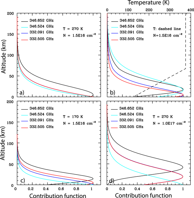
Figure 12. Sample disk-averaged contribution functions for the four SO2 transitions detected in our ALMA data, based upon our uniform, hydrostatic model atmosphere. (a) Contribution functions for a column density (N t = 1.5 × 1016 cm−2) and isothermal temperature (T = 270 K) that match most of our data (Sections 4.3, 4.4). (b) A temperature profile as indicated by the dashed line. This profile is inspired by profiles affected by plasma heating from above, such as shown by Gratiy et al. (2010). Resulting line profiles do not match our data. (c) Contribution functions from panel (a) for a much colder isothermal atmosphere (T = 170 K). Resulting line profiles do not match our data. (d) Contribution functions from panel (a) for a much higher column abundance (N t = 1017 cm−2), such as expected on the anti-Jovian hemisphere. Resulting line profiles do not match our data.
Download figure:
Standard imageHigh-resolution image
4.3. SO2 on 2018 March 20: Sunlight Eclipse
4.3.1. Disk-integrated Line Profiles
We first focus on the disk-integrated line profiles of SO2 for Io in sunlight. We have five transitions; although there essentially is no signal in the weakest line transition (333.043 GHz, in spw7), it still helps to constrain the parameters. The free parameters in our model are N t, T t, fr t, _v_rot, and v r, where the subscript t is used for disk-integrated data. We thus have to find a set of parameters that can match the line profiles in all SO2 transitions. Moreover, as the fractional coverage, fr t, should match that derived from the maps, _fr_map (Table 3), the parameter fr t is heavily constrained for disk-integrated line profiles.
While the Doppler shift, v r, in our implementation leads to a shift in frequency (i.e., velocity) of the entire line profile, both the temperature and rotation of the body (or any zonal wind), _v_rot, lead to a broadening of the line profile. Hence, high values of _v_rot can be compensated by lower atmospheric temperatures. For example, for v rot = 300 m s−1 and T t = 195 K, the line shape matches the observed profiles quite well; however, for any given N t, there is not a single value for fr t that can match the line profiles for all transitions; moreover, fr t should be equal to _fr_map. Based upon such comparisons, we can rule out zonal winds much larger than ∼100 m s−1, which agrees with our earlier findings where we did not see evidence on the maps for large zonal winds, except perhaps for September 11 (Section 3.3). Because there is no noticeable broadening in the line profiles for zonal winds up to ∼100 m s−1, we ignore any potential presence of zonal winds in the rest of this section, and simply use v rot = 75 m s−1.
By assuming that the fractional coverage of SO2 on Io, fr t, should be the same for all transitions and be equal to _fr_map, we get a pretty tight constraint on the column density and atmospheric temperature: N t = (1.35 ± 0.15) × 1016 cm−2 and T t = 270 ± 5025 K. These numbers are summarized in Table 3, together with fr t; the spread in fr t between transitions is written as an uncertainty.
We found that the modeled profile had to be shifted in its entirety by +20 m s−1 (22–23 kHz), with an estimated error of 7 m s−1. Because uncertainties in the line positions as measured in the laboratory are of order 4 kHz,10 the observed offset cannot be caused by measurement errors in the lab. This shift is indicative of material moving away from us. This can be caused by an asymmetric distribution of the gas with more material on the eastern than western hemisphere. Alternatively, it can be caused by day-to-night flows or gas falling down onto the surface such as expected in volcanic eruptions after ejection into the atmosphere. The rising branch of gas plumes usually occurs over a small surface area (vent), is very dense (∼few 1018 cm−2; see, e.g., Zhang et al. 2003), and therefore saturated. While rising, the plume cools and expands, and the return umbrella-like flow, essentially along ballistic trajectories, covers a much larger area, up to hundreds of kilometers from the vent, with column densities about two orders of magnitude lower than at the vent. Hence, as the downward flow covers a much larger area than the rising column of gas, one can qualitatively explain a redshift of disk-integrated line profiles. This idea was used by Lellouch et al. (1994; see Lellouch 1996 for updates) to explain ∼80 m s−1 redshifts in their line profiles, which they could model if there would be of order 50 plumes on the observed hemisphere. Although this seemed quite a large number of plumes at the time, if one considers the presence of stealth plumes (Johnson et al. 1995) and the recent publication of the spatial distribution of 1.707 _μ_m SO emissions (de Pater et al. 2020), this may be a quite plausible idea.
Several fits are shown in Figure 13, panels (a) and (c). For each of the models shown, we used the mean fractional coverage as derived from the line profiles in the four spectral windows (spw1, spw2, spw5, and spw6) for that particular model, i.e., fr t = 0.32 for the best-fit model (N t = 1.35 × 10¹⁶), but fr t = 0.39 for N t = 1 × 1016 cm−2 and fr t = 0.26 for N t = 2 × 1016 cm−2. While all three model curves might match one or two spectral windows, only one curve (red one) fits all transitions, as well as _fr_map. Note, though, that none of the curves fits the broad shoulders of the observed profiles; this is clearly caused by the relatively high velocities (Doppler shift) of the eruptions, as discussed in Section 3.3 and Figure 9.
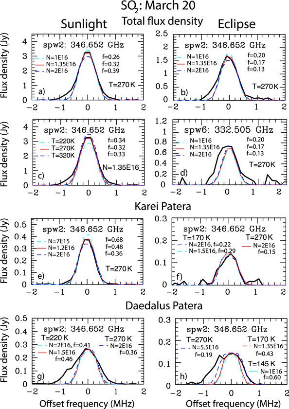
Figure 13.
SO2 line profiles (in black) with superposed various models. The red lines show the best-fit models. All panels show data and models at 346.652 GHz (spw2), except for panel d. (a) Disk-integrated flux density for Io in sunlight, with the best-fit (N t = 1.35 × 1016 cm−2) model superposed at the best-fit temperature T t = 270 K, and a fractional coverage fr t = 0.32 (in red). Several models are shown to provide a sense of the accuracy of the numbers; the fractional coverage for these models is indicated on the right side of the line profile. (b) Disk-integrated flux density for Io in eclipse, with the best fit (N t = 1.35 × 1016 cm−2), T t = 270 K, fr t = 0.17 (in red) superposed. (c) Same as panel (a) to show the sensitivity to the temperature. (d) Same as panel (b), but at 332.505 GHz (spw6). (e)–(h) Data for Karei and Deadalus Paterae, integrated over 1 beam diameter (in black). Various hydrostatic models are superposed, as indicated. The complete figure set shows the line profiles in the five spectra windows. (The complete figure set (6 images) is available.)
Download figure:
Standard imageHigh-resolution image
The column density and temperature hardly change for Io in eclipse (scans 11+15; Table 3). The drop in flux density is mainly caused by the factor of ∼2 drop in fractional coverage. In other words, a smaller fraction of the satellite is covered by gas, but over those areas, the column density and temperature are essentially the same as those seen on Io in sunlight. Line profiles are shown in panels (b) and (d) of Figure 13. We note the discrepancy between the data and models in panel (d), indicative of shortcomings in our model: while the line profiles of Io in sunlight can be modeled relatively well with our simple hydrostatic model, the model falls short when the gas emissions are dominated by volcanic plumes rather than by SO2 sublimation. In this particular case, there appears to be excess emission at lower frequencies, i.e., at velocities moving away from us.
4.3.2. Line Profiles for Individual Volcanoes
We next investigate the line profiles of individual volcanoes, Karei and Daedalus Paterae. These line profiles were created by integrating over a circle with a diameter equal to the HPBW (Table 2) centered on the peak emission of the volcano on the 346.652 GHz (spw2) map. We determined the line profile for the models in the exact same way, so that the rotation of the satellite was taken into account, and the viewing geometry (i.e., the path length through the atmosphere) was the same. Hence, the modeled line profile for a volcano on the west (east) limb is already Doppler-shifted to account for the satellite’s rotation toward (away from) us, and any additional shifts are intrinsic to the volcano itself. As shown, the hydrostatic line profiles match the observed spectra for Karei Patera in sunlight very well (Figure 13(e)) with column density and temperature quite similar to the numbers we found for the integrated flux densities, but with a fractional coverage of almost 50% (Table 4). Hence, the column density (cm−2) of SO2 gas in sunlight appears to be quite constant across Io over areas where there is gas, i.e., over approximately 30%–35% of Io’s surface in sunlight, and over about half the area of a volcanically active source (note that we integrated here over approximately the size of the beam, so the plume itself may be unresolved).
**Table 4.**Analysis of SO2 Line Profiles for Individual Volcanoes
| Date | Volcano | fr _v_a | N _v_a | T _v_a | v r,_v_a | Comments |
|---|---|---|---|---|---|---|
| (%) | (×1016 cm−2) | (K) | (m s−1) | |||
| 03-20 | Karei P. | 48 ± 2 | 1.2 ± 0.3 | 270 ± 40 | +60 ± 7 | sunlight |
| 03-20 | Karei P. | 15 ± 2 | 2 ± 0.5 | 270 ± 50 | +60 ± 10 | eclipse, scan 11+15 |
| 03-20 | Daedalus P. | 46 ± 1 | 1.5 ± 0.2 | −40 ± 7 | sunlight | |
| 03-20 | Daedalus P. | 40 ± 10 | 1.5 ± 1 | −40 ± 20 | eclipse, scan 11+15 | |
| 09-02 | P207 | 61 ± 1 | 1.2 ± 0.2 | 220 ± 25 | 0 | sunlight, set 2 |
| 09-02 | P207 | 25 ± 10 | 2 ± 1 | 250 ± 50 | 0 | eclipse, scan 6 |
| 09-02 | Nyambe P. | 55 ± 10 | 1 ± 0.3 | 270 ± 50 | 0 | sunlight, set 2 |
| 09-02 | Nyambe P. | 20 ± 5 | 1 ± 0.3 | 270 ± 50 | 0 | eclipse, scan 6 |
Note.
aColumn density N v, temperature T v, fractional coverage fr v, and radial velocity v r,v for individual volcanoes. However, note that the models are hydrostatic models, i.e., not particularly well suited for active volcanoes.
Download table as: ASCIITypeset image
Because we cannot determine the fractional coverage for individual volcanoes from the maps, we have to solely rely on finding models that give us the same fractional coverage in all four transitions. The uncertainty in fr v (the subscript v stands for volcano) as listed in Table 4 shows the spread in fr v between the four transitions. If the spread is small, the solution is quite robust. When the spread is large, the results should be taken with a grain of salt. The line center is offset by +60 m s−1, indicative of material moving away from us, such as might be expected for an umbrella-shaped plume as discussed above. The in-eclipse profile (panel (f)) can also be matched quite well, with a similar temperature, perhaps a higher column density, but a much lower fr v.
The observed profile for Daedalus Patera in sunlight is very different. The profiles in all four transitions have a pronounced red wing (Figure 13(g)). The main profile can be matched quite well with T v ≈ 220 K, and N v ≈ 1.5 × 1016 cm−2, with a fractional coverage of 46%. The line center appears to be Doppler-shifted by −40 m s−1, i.e., material moving toward us. Note that the line offsets for the two volcanoes are in the direction of a retrograde, rather than prograde, zonal wind; however, if such a wind would prevail, we would expect the wind speed to be largest near the limb (Daedalus Patera), i.e., opposite to the observations. The observed Doppler shifts are more likely local effects, produced by the eruptions. For the in-eclipse profile (Figure 13(h)), no good solution could be found, as indicated by the large uncertainties. This is not too surprising, as in eclipse, most emissions are likely volcanic in origin, because as soon as SO2 gas is cooled to below its condensation temperature, it may condense out. The applicability of our simple hydrostatic model is therefore limited. To properly model these, one needs to add volcanic plumes to the model, such as done by, e.g., Gratiy et al. (2010). (See also Section 5.3).
4.4. SO2 on 2018 September 2 and 11: Eclipse sunlight
Figure 14 shows several line profiles for the September data; best fits are summarized in Tables 3 and 4. As with the March data, the disk-integrated line profiles for both September 2 and 11 for Io in sunlight can be modeled quite well with our simple hydrostatic model, in contrast to line profiles taken of Io in eclipse where emissions must be volcanic in origin, and the applicability of our model is limited. From our hydrostatic models, we find that the SO2 fractional coverage on both days is a factor of 3 lower for the in-eclipse data than for Io in sunlight, while it was only a factor of 2 in March. On the latter date, the satellite had only been in shadow, though, for 15 minutes, much shorter than for the September data. While on September 11, the column density between in-sunlight and in-eclipse data is very similar, on September 2 it may be a factor of 2 higher when in eclipse, although the uncertainties are large enough to accommodate no change as well.
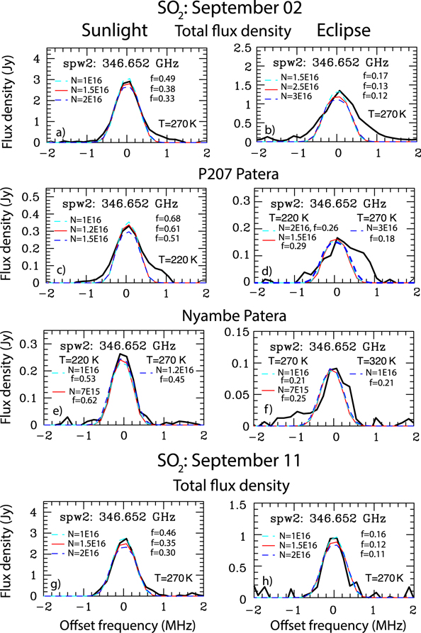
Figure 14.
SO2 line profiles (in black) with various models superposed. The red lines show the best-fit models. All data and models are at 346.652 GHz (spw2). The temperature (T), column density (N), and fractional coverage (fr) are indicated for each model. Panels (a)–(f) are for September 2, (g)–(h) for September 11. (a) Disk-integrated flux density for Io in sunlight. b) Disk-integrated flux density for Io in eclipse. (c)–(d) Line profiles for P207 Patera in sunlight and in eclipse. (e)–(f) Line profiles for Nyambe Patera in sunlight and in eclipse. (g)–(h) Line profiles for the total flux density for September 11 in sunlight and in eclipse, respectively. The complete figure set shows the line profiles in the five spectra windows. (The complete figure set (8 images) is available.)
Download figure:
Standard imageHigh-resolution image
Line profiles of individual volcanoes, calculated by integrating over a circle with a diameter equal to the HPBW, also deviate significantly from the hydrostatic models, although for volcanoes in sunlight, the discrepancies are smaller than when they are in eclipse. We were able to find a good model for P207, in particular in sunlight, where a column density quite similar to that found for the disk-integrated line profiles covers ∼60% of the volcano. During eclipse, the fractional coverage decreases by a factor of ∼2 (or more), while the column density may not vary much (considering the uncertainties). In contrast, even though the observed line profiles for Nyambe Patera look quite Gaussian both in sunlight and in eclipse, we were not able to find a model for either data set with the same fr v for all four transitions, which translates into a high uncertainty even for the in-sunlight data.
4.5. SO Line Profiles
We modeled the disk-integrated SO line profiles in Figure 15 by adopting the temperature that was determined from the SO2 profiles on the various days, because the atmospheric temperature should not depend on the species considered. The fractional coverage as determined from the line center maps for Io in sunlight is about a factor of 2 lower for SO than for SO2 in March, and more like a factor of 3–4 in September. The temperature together with this fractional coverage should result in a trustworthy value for the column density, assuming again that the atmosphere is in hydrostatic equilibrium. With these assumptions, we find a column density of ∼1015 cm−2 on March 20 when in sunlight, roughly a factor of 10 below the SO2 column density. This, with the lower fractional coverage, suggests a difference of a factor of ∼20 between the total volumes of SO and SO2 gas, in good agreement with previous observations (e.g., Lellouch et al. 2007). On September 2, the column density is roughly a factor of 5 lower than the SO2 column density, which with the much lower fractional coverage also suggests almost a factor of 20 difference in gas volumes. On September 11, the column density is again a factor of 10 below the SO2 value, but with a much lower fractional coverage, this results in a difference of ∼40 between the volumes of SO2 and SO gases.
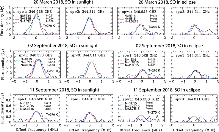
Figure 15. SO line profiles (in black) with superposed various hydrostatic models. The red lines show the best fits; all models shown are at 346.528 GHz (spw1) and 344.311 GHz (spw3). The temperature (T), column density (N), and fractional coverage (fr) are indicated for each model. The dates are indicated above each row. Note the shape of the profiles and the variations in intensity.
Download figure:
Standard imageHigh-resolution image
As shown in Figures 4, 6, 7, and 15, we did detect SO when Io was in eclipse in March and on September 2, but not on September 11. The S/N in the maps, however, is very low, which prevented a good estimate of the fractional coverage, a necessary quantity to determine the column density from the data. Assuming the same temperature as derived from the SO2 maps for Io in eclipse, we find a fractional coverage of 7% for an SO column density of 1015 cm−2, i.e., about half the fractional area for the same column density as seen in the in-sunlight maps. The fractional coverage decreases for a higher value of N t, and vice versa for a lower value. On September 2, the most likely scenario for Io in eclipse is that both fr t and N t decrease by a factor of 2, while on September 11 no SO emissions were detected in eclipse.
5.1. Summary of Observations
We observed Io with ALMA in Band 7 (880 _μ_m) in five SO2 and two SO transitions when it went from sunlight into eclipse (2018 March 20), and from eclipse into sunlight (2018 September 2 and 11). On all three days, we obtained disk-resolved data cubes and analyzed SO2 and SO line profiles for both the disk-integrated data and for several active volcanoes on the disk-resolved data cubes. Specifics on the observations and derived parameters are summarized in Tables 1–4.
5.1.1. Disk-integrated Data: SO2
The line-emission disk-integrated flux densities11 are typically ∼2×–3× higher for Io in sunlight than in eclipse (Figure 5), indicative of a roughly 30%–50% contribution of volcanic gases to the SO2 emissions. However, there is much variability in these numbers. On September 11, the SO2 flux density in sunlight was 4–5 times higher than in eclipse. In March, when Io went into eclipse, the flux density in the strongest transition, _F_346.652, dropped exponentially by a factor of 3, in contrast to the factor of 2 drop in the three weaker transitions. _F_346.652 for Io in sunlight was ∼2× higher than _F_346.524, about 30% above the ratio in their intrinsic line strengths (Table 1). In contrast, the observed ratios between _F_346.524 with _F_332.091 and with _F_332.505 are 40% and 60% smaller than the ratios between their intrinsic line strengths. As the flux density in the various transitions depends also on the atmospheric temperature, which determines (in LTE) which energy levels in the molecule are populated (Boltzmann’s equation), the differences in flux density between the various transitions were used in Section 4 to determine the column density and atmospheric temperature. For example, for lower temperatures, the modeled _F_346.652 would be too low, while the modeled _F_332.505 would be too high, which can be qualitatively understood from the difference in contribution functions between panels (a) and (c) in Figure 12. We found that neither the atmospheric temperature nor the column density between the in-sunlight and in-eclipse data sets noticeably changed, but that the differences in flux density could be accounted for by a factor of 2–3 decrease in fractional coverage. In other words, the column densities (cm−2) remained the same, but there were fewer areas (two to three times less) above which SO2 gas was present.
Tsang et al. (2016) measured a factor of 5 ± 2 drop in column density when Io moved from sunlight into eclipse. However, because they cannot distinguish between a high column density with low fractional coverage and a low column density with a high fractional coverage, our findings essentially agree.
All observations could be matched quite well with an isothermal atmospheric temperature of 270 ± 50 K. This is clearly an oversimplification, as the temperature will certainly vary with altitude, and also with latitude, longitude, and time of day. Walker et al. (2010) showed that the atmospheric (translational) temperature rises steeply with altitude due to plasma heating from above. Near the surface, the SO2 gas is expected to be in equilibrium with the surface frost, rising to ∼400 K at an altitude of 70 km during the day; at night, the plasma can reach lower altitudes so that the 400 K temperature may be reached at an altitude of ∼40 km. The exact 3D temperature profile depends on the 3D distribution of the atmospheric density, which for SO2 is tightly coupled with the frost distribution and temperature. Moreover, as seen from the previous sections, volcanic plumes may affect the atmosphere and its temperature structure quite dramatically. We will get back to this in Section 5.3. The bottom line is that altitude-dependent changes in temperature and density affect the various transitions in different ways, as shown by the contribution functions in Figure 12.
In contrast to the exponential decrease in intensity during eclipse ingress, there is a linear increase during egress for at least about 10 minutes. Interestingly, the SO2 flux density in three of the four transitions ∼10 minutes after emerging from eclipse on September 2 is higher than the values a half hour later: 4% ± 2.6% higher for _F_346.652, 16% ± 7% for _F_332.091, and 19% ± 7% for _F_332.505.
The disk-integrated flux densities for September 11 are shown alongside the September 2 numbers in Figure 5. The in-eclipse flux densities for SO2 on September 11 are typically a factor of 2 (two strongest transitions) to 3 (two weakest transitions) below the September 2 in-eclipse values. As shown in the line center maps, on September 11, the volcanic activity was very low, which may explain the difference in flux densities between these dates. When in sunlight, the September 11 numbers for SO2 are well below the September 2 values, in particular for the two weakest transitions, which are lower by a factor of 1.18 ± 0.09 at 332.091 GHz and 1.29 ± 0.09 at 333.043 GHz compared to the nearby high September 2 values.
Because all SO2 at temperatures below its dew point (i.e., near the surface) condenses out, only gas sourced from volcanic vents, or SO2 gas that was prevented from complete collapse by a layer of noncondensible gases (e.g., Moore et al. 2009), can be present on Io in eclipse. These gases apparently cover ∼10%, and at times up to almost 20% of Io’s surface. In some cases, there is a clear connection to a particular volcanic eruption; in other cases, emissions from volcanically sourced gases could be caused by stealth volcanism, the presence of which had been postulated to explain the 1.707 _μ_m forbidden emissions on this hemisphere (de Pater et al. 2020). Point sources and glows of gases that were seen on this hemisphere with the New Horizons spacecraft, interpreted as being caused by plasma interactions with the (near-)surface (Spencer et al. 2007), could also be a signature of stealth volcanism (de Pater et al. 2020).
5.1.2. Disk-integrated Data: SO
The SO flux density for Io in sunlight is highest on September 2 (0.66 ± 0.03 Jy) and lowest on September 11 (0.45 ± 0.04 Jy). Despite the fact the SO is not expected to significantly decrease during an eclipse (Section 3.2), we see a gradual (linear) decrease by a factor of 2 in March. Because SO does not condense at these temperatures, it is likely removed from the atmosphere through reactions with itself on the surface, at a much faster rate than hitherto anticipated (Section 3.2). SO similarly is restored much more slowly than SO2, indicative of formation from SO2 through photolysis. According to Moses et al. (2002), SO is formed through photolysis of SO2 at a column abundance rate of 4.6 × 1011 cm−2 s−1, i.e., it takes about a half hour to produce a full column of ∼1015 cm−2 s−1. Above volcanoes, about 50% of SO is produced this way, and another 50% may be produced at a similar rate through the reaction of O+S2. The data (Figure 5) show that SO is fully restored within ∼10 minutes of time, which, given the uncertainties in the ALMA column densities and the various processes to produce SO (Section 3.2), agrees pretty well with the models.
5.1.3. Disk-resolved Data and Line Profiles
On March 20, the SO2 emission is dominated by the volcanically active Karei and Daedalus Paterae, while some low-level emission is seen near North Lerna. On September 2, the emission is dominated by P207, while we also see emission near PFd1691 and Nyambe Patera. The situation is less clear on September 11: P207 Patera was no longer active, while emissions on Io in sunlight were seen above Karei and Nyambe Paterae. In-eclipse very low-level activity was seen over Karei, Gish Bar, Ra and P129 Paterae, north of P207, and near Euboea Fluctus. SO emissions in March tracked the SO2 emissions reasonably well, i.e., both Karei and Daedalus Paterae showed activity. On September 2, no clear SO emissions were seen during eclipse, but ∼4 minutes after Io emerged from eclipse, SO emissions were detected over P207 and near Nyambe Paterae. On September 11 no SO emissions were detected in eclipse; when Io was in sunlight, SO emissions were highest over Karei Patera, and visible above P129 and faintly across the equatorial band, more or less coinciding with the SO2 emissions. This all suggests that the main source of SO is photolysis of SO2. As mentioned above, at volcanic eruption sites, a full column of ∼1015 cm−2 s−1 will be produced in 15 minutes. The SO peak intensity levels above P207 changed from ≲0.04 Jy/bm in eclipse (scan 6, Figure 6), to ∼0.07 Jy/bm (sc. 8) to ∼0.12 Jy/bm in sunlight. Hence, in ∼4 minutes, photochemical reactions likely produce enough SO to explain the observations.
The effect of volcanoes on the SO2 and SO emissions is most clearly seen in the line shapes. While disk-integrated Io-in-sunlight data can usually be matched quite well with hydrostatic models, the in-eclipse profiles deviate considerably from such Gaussian-shaped profiles. Both in-sunlight and in-eclipse disk-integrated line profiles show broad low-level wings out to ∼1 MHz from line center, indicative of velocities of order 800–900 m s−1 both toward and away from the observer. As shown on Figures 9 and 10, these wings are clearly caused by volcanic plumes.
The line profiles for individual volcanoes often show red- or blueshifted shoulders or wings, while on some occasions, the entire profile seems to be shifted toward lower or higher frequencies. In particular in March, the SO2 line profile of Karei Patera showed a +60 m s−1 shift, and a −40 m s−1 shift for Daedalus Patera, while the disk-integrated line profiles were redshifted by +20 m s−1. Based upon our earlier discussions, the redshifts may be caused by the plume above Karei Patera, where ejection of the gas is confined to a small (unresolved) area, while the plume material falls back down on the surface over a much larger area, hundreds of kilometer in radius, resulting in a redshift in the line profile. Daedalus Patera, showing a blueshift (which in part offsets the redshift in the disk-integrated line profile), must be dominated by material moving toward us. Daedalus, in contrast to Karei Patera, is located very close to Io’s limb (Figure 4) and hence is seen under a very different viewing geometry such that not only the rising plume material but also part of the umbrella-shaped plume is moving toward us, resulting in a blueshift of the entire profile. The redshifted wing on the volcano’s line profile is still indicative of material falling down onto the surface, away from us, much of it perhaps over the limb.
The emission over P207 is also on the limb of the satellite, but here we see a wing or shoulder of blueshifted material while there is no noticeable offset of the entire profile. Clearly, both the viewing geometry and the exact geometry or shape of the plume and ejection itself, in combination with overall wind-flow patterns (e.g., Gratiy et al. 2010), are important parameters that affect the line profile.
5.2. Post-eclipse Brightening
As mentioned above, the flux density on September 2 ∼10 minutes after emerging from eclipse was considerably higher, up to ∼20% in some transitions, than half an hour later. This appears to be an anomalous post-eclipse brightening effect. A ∼10% brightening of the satellite for about 10–20 minutes after emerging from eclipse was first reported by Binder & Cruikshank (1964) at a wavelength of 450 nm, i.e., they observed the satellite’s surface in reflected sunlight. The authors noted that Io was ∼10% brighter when it emerged from eclipse, which decreased over the next ∼15 minutes. They suggested that the brightening might be caused by an atmospheric component that condenses on Io’s surface during the eclipse. This makes the satellite bright; the ice should evaporate only minutes after receiving sunlight again, resulting in a slow darkening, back to its original reflected-sunlight intensity. We note that these observations were obtained before Io’s atmosphere and its volcanic activity were detected—in fact, based on their data, the authors suggested Io having an atmosphere. During subsequent years, both detections and nondetections (e.g., Cruikshank et al. 2010; Tsang et al. 2015) of this “post-eclipse brightening” effect have been reported at wavelengths from the UV to the mid-IR. Explanations of the effect range from condensation with subsequent sublimation of SO2 frost (Binder & Cruikshank 1964; Fanale et al. 1981; Bellucci et al. 2004), to changes in Io’s reflectivity due to sulfur allotropes as a result of changes in surface temperature (Hammel et al. 1985), to interactions of atmospheric molecules with Jupiter’s magnetospheric plasma (Saur & Strobel 2004). Some authors concentrate on phenomena causing a brightening of the surface, and others those of the atmosphere. No clear explanation has been provided yet; as shown by the data, the effect has not always been detected, which has been interpreted as due to possible differences in frost coverage at different longitudes.
The gradual increase in flux density in our data during the first ∼10 minutes after emerging from eclipse into sunlight is exactly how Binder & Cruikshank (1964) explained their observed post-eclipse brightening of Io’s surface: the surface was bright because the SO2-ice coverage had increased due to condensation while in eclipse; as soon as the surface warmed, SO2 sublimed, the satellite’s surface darkened, and the atmosphere re-formed. The situation, as we observed it, is a bit more complex in that we see the SO2 flux density to “overshoot” after 10 minutes (the end of our observing session 1 on September 2), before reaching a steady state (in observing set 2 on September 2). In the next section ,we show that this may result from the interaction of volcanic plumes with the re-forming atmosphere.
5.3. Comparison of Data with Atmospheric Models
In Section 5.3.2, we compare the above results with simulations of volcanic plumes by Zhang et al. (2003) and McDoniel et al. (2017). Before doing so, we summarize those authors’ simulations in the next Section.
5.3.1. Summary of Published Plume Simulations
McDoniel et al. (2017) coupled Zhang et al.'s (2003, 2004) original plume model to a model of a sublimation-driven atmosphere, developed over the years by Moore et al. (2009) and Walker et al. (2010, 2012). These simulations include a fulltreatment of gas dynamics, radiation (heating and cooling through rotational and vibrational radiation), sublimation, and condensation. Simulations with this coupled model show how a volcanic plume on the day side expands in a sublimating atmosphere. The authors present models for a Pele-type plume both on the night and day side. They assumed a night-side surface temperature of 90 K and 116–118 K during the day. The gas erupts from the vent at a temperature of ∼600 K and a source rate of ∼1029 SO2 molecules s−1 at hypersonic velocities of close to 1 km s−1. It then expands and cools. At an altitude of ∼300 km, a canopy-shaped shock forms (due to Io’s gravity field), where the radially expanding molecules turn back down to the surface. Most of the gas falls down ∼400–600 km from the vent. On the night side, the SO2 gas condenses and forms a ring around the volcano which matches the red ring observed around Pele. Due to plume expansion and vibrational cooling, the gas temperature above the vent decreases to very low (∼50 K) temperatures, while the temperature in the canopy shock is of order 300–400 K.
On the night side, the model shows an average column density N v = 1.1 × 1016 cm−2 over a region up to ∼600 km from the vent. Directly above the vent, though, N v ≈ 1018 cm−2 and drops by an order of magnitude over a 30-km distance.
A Pele-type plume on the day side is different because there is also SO2 sublimation from Io’s surface and hence the plume expands in a background atmosphere. The extent to which a day-side sublimation atmosphere is affected by plumes depends on the size, density, and ejection velocity of the plume, as well as on the density of the sublimation atmosphere, which is set by the temperature of the surface frost (for details, see McDoniel et al. 2017). Plumes that do not rise up above the exobase (i.e., the altitude at which the mean free path length between collisions is equal to one atmospheric scale height, which is typically at an altitude of ∼30–50 km on Io; McDoniel et al. 2017) will not affect the atmosphere very much. Once a plume rises above the exobase, like a large Pele-type plume, it will produce a canopy shock similar to that on the night side. However, whereas at night the gas falls down and hits the surface, during the day, it will encounter the atmosphere, and a reentry shock develops. This will heat the atmosphere up to levels similar to or higher than that seen at the vent. The resulting high temperature will lead to excess frost sublimation, which gets entrained in the plume flow. Due to the high pressure created by the high temperature, material will be pushed away, which actually results in a decrease in the column density at the intersection between the canopy and the atmosphere (i.e., where at night the red ring around Pele was created). Some of the material falling down onto the atmosphere creating the reentry shock will “bounce” once, or perhaps multiple times, back up and outwards, forming reentry shocks every time when falling down onto the atmosphere (compare, e.g., the bounces on the atmosphere seen during the Comet Shoemaker-Levy 9 impact; Nicholson et al. 1995). This expands the area of the plume’s interaction with the atmosphere by factors of 2–3. The bounces and outward expansion are more pronounced at higher surface temperatures and atmospheric densities. Because ultimately the temperature of the surface frost will maintain the hydrostatic atmosphere in vapor pressure equilibrium, the total mass in the lower atmosphere may not change much, but large amounts of plume material may displace the originally “sublimated” gas. The total mass of the material in the plume area will be enhanced, though it is not a simple addition of the sublimated atmosphere and the plume material ejected in the absence of a sublimation atmosphere (only 60%–75% of such a night-side plume is added to the sublimation atmosphere; McDoniel et al. 2017).
5.3.2. Comparing ALMA Data with Atmospheric Simulations
_Sublimation atmosphere_—During eclipse ingress in March, the SO2 flux density decreased exponentially, caused by a decrease in the volume of SO2 molecules (assuming a hydrostatic atmosphere, we showed that the column density and temperature did not change much; only the fractional area decreased). With such a tenuous atmosphere, one would expect the surface temperature to drop instantaneously when entering eclipse, as shown to be true by Tsang et al. (2016). Given a diffusion time of 70 s (Section 3.2.1; de Pater et al. 2002), the SO2 molecules are expected to rapidly condense onto the surface, which means that the number density of molecules just above the surface decreases, resulting in a downward motion of gas above it. Moore et al. (2009) show that changes occur primarily in the bottom 10–20 km. They further show that even a small amount of noncondensible gases will form a diffusion layer near the surface. Once this layer is several mean free path lengths thick, it will prevent or at least slow down further collapse of the SO2 atmosphere. They predict this to happen after about 10–20 minutes. They also predict that in this case, the gas column density and the atmospheric temperature remain essentially the same. In their calculations, they assumed, though, that SO is noncondensible, while our data show that SO in essence rapidly condenses through self-reactions on the surface (the flux density or volume of SO molecules decreases linearly at a rate of 15 mJy minute−1). However, because our observations show essentially no change in column density and temperature, and some SO2 gas is always present, even when volcanic activity is low (Figure 11), atmospheric collapse may indeed be retarded by a diffusive layer of noncondensible gases near the surface. We cannot exclude the possibility of SO2 emissions due to stealth volcanism, however.
During eclipse egress in September, both the SO2 and SO emissions increase linearly, though SO is clearly delayed compared to SO2, which we attributed to formation through photochemistry (Section 5.1.2). The atmosphere is restored within about 10 minutes after reemerging in sunlight. This suggests that the surface heats up essentially instantaneously, causing SO2 ice to start to sublimate immediately. This is very different from the calculations by Moore et al. (2009), who show the atmosphere to re-form on a much (≳3×) longer timescale.
_Volcanic plumes_—The beam size in our data is ∼1200 km, which is similar to the plume extent of Zhang et al.'s (2003) simulated Pele-type plume at night. A day-side Pele-type plume, though, when including the effect of bounces, would be resolved in our data. On September 2, when Io was in eclipse after having been ∼2 hr in the dark, the volcanic plume over P207 was quite bright, and the line profile very asymmetric (Figure 14) with a strong blueshifted component, indicative of material moving in our direction. Such a line profile would be expected from Zhang et al.'s (2003) models, as shown by Moullet et al. (2008), who calculated line profiles based upon these models at different locations on Io’s disk. Depending on the exact geometry of the plume, they find kinks or shoulders in the line profile, not unlike what we observed for P207. The blueshifted shoulder is caused by the umbrella-shaped plume material, seen on the limb, moving in our direction. The model also predicts velocities v r of order 700 m s−1, which agrees well with the wings in our disk-integrated line profiles, which are caused by the plumes (Figures 9, 10).
Within 1–2 minutes after emerging in sunlight, the P207 plume increased in intensity and continued to increase for the next several minutes (Figure 6). During this period, the plume transitions from a night-side plume to a day-side plume, when SO2 sublimation from SO2 frost becomes important. McDoniel et al. (2017) show calculations of a plume transitioning from the night to the day side, and back into the night, a process that takes almost a full Io day (42.5 hr). The ALMA observations, in contrast, show a very accelerated process because eclipse egress only takes a few minutes. During these few minutes, SO2 frost starts to sublime and the atmosphere re-forms, while the volcano continues to eject gases. The plume starts to interact with the atmosphere while it is forming. A reentry shock forms where the plume material hits the atmosphere. The resulting high temperature (Section 5.3.1) accelerates SO2 sublimation, which gets entrained in the plume flow, causing the plume area to grow. Hence, the observed brightening and expansion of the SO2 emissions near volcanic vents, i.e., near regions where we see some (though sometimes faint) SO2 emissions during eclipse, are consistent with McDoniel et al.'s simulations. It may also cause the post-eclipse brightening effect we see about 10 minutes after eclipse egress, where the sudden change from night to day and the interaction of the plume with the re-forming atmosphere may lead to a temporary “excess” in SO2 emissions, likely due to an altitude-dependent temporary increase in atmospheric temperature.
The authors further show that the average column density over the vent at night is ∼1016 cm−2, and that during the day, the column density over the plume matches that over the day-side hemisphere at distances ≳150 km. This essentially agrees with our observations, where column densities over the plume and background atmosphere on the day side are very similar. The differences in brightness we see between the day and night (eclipse) side, both disk-averaged and over volcanoes, are mostly explained by changes in the fractional area covered by the gas, but columns of gas over these areas are very similar. Given our relatively low spatial resolution, this may well be consistent with the models.
The temperature that best matches our line profiles, ∼220–320 K, can be explained qualitatively by the various temperatures expected along the line of sight through the model, which vary from ∼50 K above the vent up to 300–400 K at the canopy shock. For comparison, when Moullet et al. (2008) parameterized the Zhang et al. (2003) night-side plumes at a location ∼40° away from disk center, they found that the models could be mimicked well with an isothermal temperature of ∼190 K. However, given how complex the plume–atmosphere interaction is (McDoniel et al. 2017), we do not think that the atmosphere can be modeled correctly using a simple isostatic atmosphere.
In March we detected vigorous eruptions at Karei and Daedalus Paterae. At Karei Patera, the fractional coverage in sunlight was roughly three times larger than in eclipse, with an atmospheric temperature of 270 ± 50 K both in sunlight and in eclipse. As mentioned before, the entire profile was redshifted by 60 m s−1, while in eclipse, the profile was slightly skewed, peaking more at the blue side of the spectrum. The overall shift toward the red is indicative of plume material falling back down onto the surface, away from us; because the umbrella-shaped plume is much larger in extent than the rising column of gas, this can qualitatively explain the line profiles.
Daedalus Patera, in contrast, shows a strong redshifted shoulder, somewhat similar to the blueshifted shoulder for P207 in September. The entire profile was slightly blueshifted, presumably because the umbrella-shaped plume material from a volcanic ejection near the limb has a large component of material moving toward us (i.e., similar to the material that explains the blueshifted wing of the line for P207). The redshifted wing, though, shows that a large component of plume material is also moving away from us.
When Moullet et al. (2008) modeled the Zhang et al. plumes for comparison with their radio data, they did not see such redshifted shoulders in the models. This, together with our observations of line profiles that are very asymmetric, in particular in eclipse, shows that the volcanic eruptions are much more complex than the Zhang et al. (2003) and McDoniel et al. (2017) models predict. This is not too surprising; volcanic eruptions are likely not axisymmetric and may fluctuate in ejection speed, direction, and gas content on timescales much shorter than we can capture in our observations. Yet, it is reassuring that our observations do qualitatively match many features in the model.
We used ALMA in Band 7 (880 _μ_m) to observe Io in five SO2, two SO, and one KCl transitions when it went from sunlight into eclipse (2018 March 20), and from eclipse into sunlight (2018 September 2 and 11). We summarize the main findings as follows:
- 1.
The disk-averaged brightness temperature at 0.9 mm is 93.6 ± 5.3 K (including calibration uncertainties). The observed difference of ∼3 K between all Io-in-sunlight and in-eclipse maps, together with the 22 K drop in temperature at 19 _μ_m (Tsang et al. 2016), suggests that Io’s surface is composed of a thin, low-thermal-inertia (50 J m−2 K−1 s−1/2) layer, overlying a more compact, high-thermal-inertia (320 J m−2 K−1 s−1/2) layer, indicative of a thin (≲few millimeters) layer of dust or fine-grained volcanic deposits overlying more compact layers of rock and/or coarse-grained/sintered ice. - 2.
The SO2 and SO disk-integrated flux densities are typically about two to three times higher on Io in sunlight than in eclipse, indicative of a 30%–50% volcanic contribution to the emissions. - 3.
During eclipse ingress, the SO2 flux density dropped exponentially, with the 346.652 GHz transition (strongest line intensity) faster and more than the other transitions. Following eclipse egress, the SO2 flux densities increased linearly, with the 346.652 GHz transition faster than the others. - 4.
Eclipse egress observations show that the atmosphere is reinstated on a timescale of 10 minutes, consistent with the interpretation of the post-eclipse brightening effect reported for observations of Io’s surface reflectivity. An atmospheric post-eclipse brightening was seen in several SO2 transitions, where the flux density was up to ∼20% higher 10 minutes after reemerging in sunlight compared to a half hour later. - 5.
We attribute the variations in emissions and differences between line transitions during eclipse ingress and egress, as well as the atmospheric post-eclipse brightening effect to altitude-dependent changes in temperature, likely caused in/by volcanic plumes and their interaction with the atmosphere, such as simulated by McDoniel et al. (2017). - 6.
The SO flux density dropped/increased linearly after entering/reemerging from eclipse, in both cases clearly delayed compared to SO2. This provides confirmation that SO may be rapidly removed through reactions with Io’s surface once in eclipse, and that photolysis of SO2 is a major source of SO. - 7.
Spectral image data cubes reveal bright volcanic plumes on March 20 and September 2; no plumes were detected on September 11. Plumes on the limb create high-velocity wings in the disk-integrated line profiles (at ≳600 kHz, or ≳500 m s−1). Such high velocities match those predicted in plume simulations by Zhang et al. (2003) and McDoniel et al. (2017). - 8.
In addition to the few obvious volcanic plumes in our spectral image data cubes, the low-level SO2 emissions present during eclipse may be sourced by stealth volcanic plumes or be evidence of a layer of noncondensible gases, preventing the complete collapse of SO2, as modeled by Moore et al. (2009). - 9.
Based upon hydrostatic model calculations, typical disk-integrated SO2 column densities and temperatures are N t ≈ (1.5 ± 0.3) × 1016 cm−2 and T t ≈ 220–320 K both for Io in sunlight and in eclipse. SO column densities are roughly a factor of 5–10 lower. The main differences between in-sunlight and in-eclipse flux densities appear to be caused by a factor of 2–3 smaller fractional coverage in eclipse (i.e., down from 30% to 35% SO2 and ∼12% SO in sunlight). - 10.
The active volcanoes on March 20 and September 2 show similar SO2 column densities and temperatures to the disk-integrated profiles, but with a very high fractional coverage (∼50%–60% in sunlight, versus 30%–35% disk averaged). This seems consistent with McDoniel et al.'s (2017) simulations, where the column densities blend into the background at distances over a few 100 km from the volcanic vent. - 11.
Line profiles of in-eclipse data are very asymmetric, both for disk-integrated profiles and individual volcanoes. Some volcanoes show redshifted, and others blueshifted, shoulders, both in sunlight and in eclipse. Sometimes, the entire profile is slightly red- or blueshifted. The line profiles must be strongly affected by the intrinsic properties of volcanic plumes (e.g., ejection speed, direction, density, and variations therein), in addition to their viewing geometry. - 12.
The data are suggestive of a 300–400 m s−1 horizontal prograde wind on September 11, when no volcanic activity was reported; however, such a wind is not supported by disk-integrated line profiles. No zonal winds were detected on March 20 and September 2, when volcanic plumes were seen. - 13.
KCl gas has only been detected on March 20, sourced mainly from near Ulgen Patera. No SO or SO2 gas was detected at this location. Hence, the magma in the chambers that power volcanoes must have different melt compositions, and/or the magma has access to different surface/subsurface volatile reservoirs. - 14.
Our data can be qualitatively explained by the night-side plume simulations of Zhang et al. (2003) and day-side simulations by McDoniel et al. (2017), although it is also clear that the data are much more complex than the models can capture.
Our observations begin to clarify the role of volcanism in forming Io’s atmosphere. However, many questions still remain, including, e.g., Io’s overall atmospheric temperature profile, in particular in the first 10–20 km above the surface; longitudinal variations in column density; winds; volcanic sources; and magma composition. Although it is clear that low-level emissions are present during eclipse, we do not yet understand the cause of these: perhaps stealth volcanism, or a layer of noncondensible gases preventing complete collapse of the SO2 atmosphere. To further address these questions, we plan to obtain ALMA data at a higher spatial resolution when the satellite is at eastern and western elongation. Future work will also need to include realistic plume models in addition to the hydrostatic models employed here.
We are grateful for in-depth reviews by David Goldstein and one anonymous referee, which helped improve the manuscript substantially. This paper makes use of ALMA data ADS/JAO.ALMA#2017.1.00670.S. ALMA is a partnership of ESO (representing its member states), NSF (USA), and NINS (Japan), together with NRC (Canada), MOST and ASIAA (Taiwan), and KASI (Republic of Korea), in cooperation with the Republic of Chile. The Joint ALMA Observatory is operated by ESO, AUI/NRAO, and NAOJ. The National Radio Astronomy Observatory is a facility of the National Science Foundation operated under cooperative agreement by Associated Universities, Inc. The data can be downloaded from the ALMA Archive. This research was supported by the National Science Foundation, NSF grant AST-1313485 to UC Berkeley. P.M.R. acknowledges support from ANID basal AFB170002.
Facility: ALMA. -