PySpark DataFrame Tutorial: Introduction to DataFrames (original) (raw)

DataFrames is a buzzword in the industry nowadays. People tend to use it with popular languages used for Data Analysis like Python, Scala, and R. So, why is it that everyone is using it so much? Let's take a look at this with our PySpark Dataframe tutorial. In this post, I'll be covering the following topics:

DataFrames generally refer to a data structure, which is tabular in nature. It represents rows, each of which consists of a number of observations. Rows can have a variety of data formats (heterogeneous), whereas a column can have data of the same data type (homogeneous). DataFrames usually contain some metadata in addition to data; for example, column and row names.

We can say that DataFrames are nothing, but 2-dimensional data structures, similar to a SQL table or a spreadsheet. Now let's move ahead with this PySpark Dataframe Tutorial and understand why exactly we need Pyspark Dataframe.

Why Do We Need DataFrames?

1. Processing Structured and Semi-Structured Data

DataFrames are designed to process a large collection of structured as well as semi-structured data. Observations in Spark DataFrame are organized under named columns, which helps Apache Spark understand the schema of a Dataframe. This helps Spark optimize the execution plan on these queries. It can also handle petabytes of data.

2. Slicing and Dicing

DataFrames APIs usually support elaborate methods for slicing-and-dicing the data. It includes operations such as "selecting" rows, columns, and cells by name or by number, filtering out rows, etc. Statistical data is usually very messy and contains lots of missing and incorrect values and range violations. So a critically important feature of DataFrames is the explicit management of missing data.

3. Data Sources

DataFrames has support for a wide range of data formats and sources, we'll look into this later on in this Pyspark DataFrames tutorial. They can take in data from various sources.

4. Support for Multiple Languages

It has API support for different languages like Python, R, Scala, Java, which makes it easier to be used by people having different programming backgrounds.

Features of DataFrames

DataFrames are distributed in nature, which makes it a fault tolerant and highly available data structure.
Lazy evaluation is an evaluation strategy which holds the evaluation of an expression until its value is needed. It avoids repeated evaluation. Lazy evaluation in Spark means that the execution will not start until an action is triggered. In Spark, the picture of lazy evaluation comes when Spark transformations occur.
DataFrames are immutable in nature. By immutable, I mean that it is an object whose state cannot be modified after it is created. But we can transform its values by applying a certain transformation, like in RDDs.

PySpark DataFrame Sources

DataFrames in Pyspark can be created in multiple ways:

Data can be loaded in through a CSV, JSON, XML, or a Parquet file. It can also be created using an existing RDD and through any other database, like Hive or Cassandra as well. It can also take in data from HDFS or the local file system.

Let's move forward with this PySpark DataFrame tutorial and understand how to create DataFrames.

We'll create Employee and Department instances.

from pyspark.sql import *

Employee = Row("firstName", "lastName", "email", "salary")

employee1 = Employee('Basher', 'armbrust', 'bash@edureka.co', 100000)
employee2 = Employee('Daniel', 'meng', 'daniel@stanford.edu', 120000 )
employee3 = Employee('Muriel', None, 'muriel@waterloo.edu', 140000 )
employee4 = Employee('Rachel', 'wendell', 'rach_3@edureka.co', 160000 )
employee5 = Employee('Zach', 'galifianakis', 'zach_g@edureka.co', 160000 )

print(Employee[0])

print(employee3)

department1 = Row(id='123456', name='HR')
department2 = Row(id='789012', name='OPS')
department3 = Row(id='345678', name='FN')
department4 = Row(id='901234', name='DEV')

Next, we'll create a DepartmentWithEmployees instance from the Employee and Departments.

departmentWithEmployees1 = Row(department=department1, employees=[employee1, employee2, employee5])
departmentWithEmployees2 = Row(department=department2, employees=[employee3, employee4])
departmentWithEmployees3 = Row(department=department3, employees=[employee1, employee4, employee3])
departmentWithEmployees4 = Row(department=department4, employees=[employee2, employee3])

Let's create our DataFrame from the list of rows:

departmentsWithEmployees_Seq = [departmentWithEmployees1, departmentWithEmployees2]
dframe = spark.createDataFrame(departmentsWithEmployees_Seq)
display(dframe)
dframe.show()

Pyspark DataFrames Example 1: FIFA World Cup Dataset

Here we have taken the FIFA World Cup Players Dataset. We are going to load this data, which is in a CSV format, into a DataFrame and then we'll learn about the different transformations and actions that can be performed on this DataFrame.

Reading Data From CSV File

Let's load the data from a CSV file. Here we are going to use the spark.read.csv method to load the data into a DataFrame, fifa_df. The actual method is spark.read.format[csv/json] .

fifa_df = spark.read.csv("path-of-file/fifa_players.csv", inferSchema = True, header = True)

fifa_df.show()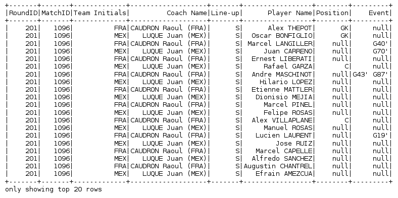

Schema of DataFrame

To have a look at the schema, i.e. the structure of the DataFrame, we'll use the printSchema method. This will give us the different columns in our DataFrame, along with the data type and the nullable conditions for that particular column.

fifa_df.printSchema()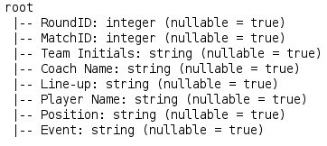

Column Names and Count (Rows and Column)

When we want to have a look at the names and a count of the number of rows and columns of a particular DataFrame, we use the following methods.

fifa_df.columns //Column Names

fifa_df.count() // Row Count

len(fifa_df.columns) //Column Count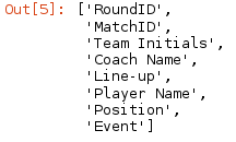

37784

8

Describing a Particular Column

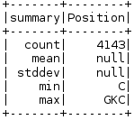
If we want to have a look at the summary of any particular column of a DataFrame, we use thedescribe method. This method gives us the statistical summary of the given column, if not specified, it provides the statistical summary of the DataFrame.

fifa_df.describe('Coach Name').show()
fifa_df.describe('Position').show()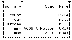

Selecting Multiple Columns

If we want to select particular columns from the DataFrame, we use the select method.

fifa_df.select('Player Name','Coach Name').show()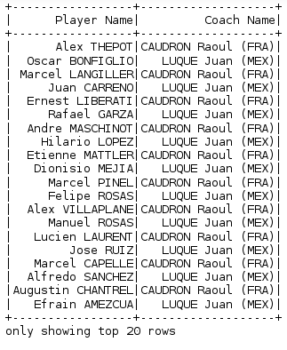

Selecting Distinct Multiple Columns

fifa_df.select('Player Name','Coach Name').distinct().show()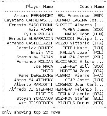

Filtering Data

In order to filter data, according to the condition specified, we use the filter command. Here we are filtering our DataFrame based on the condition that Match ID must be equal to 1096 and then we are calculating how many records/rows are there in the filtered output.

fifa_df.filter(fifa_df.MatchID=='1096').show()

fifa_df.filter(fifa_df.MatchID=='1096').count()  //to get the count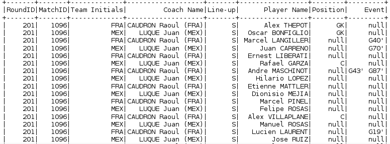

Filtering Data (Multiple Parameters)

We can filter our data based on multiple conditions (AND or OR)

fifa_df.filter((fifa_df.Position=='C') && (fifa_df.Event=="G40'")).show()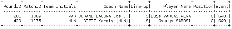

Sorting Data (OrderBy)

To sort the data we use the OrderBy method. By default, it sorts in ascending order, but we can change it to descending order as well.

fifa_df.orderBy(fifa_df.MatchID).show()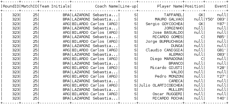

PySpark Dataframes Example 2: Superheros Dataset

Loading the Data

Here we will load the data in the same way as we did earlier.

Superhero_df = spark.read.csv("path-of file/superheros.csv", inferSchema = True, header = True)

Superhero_df.show(10)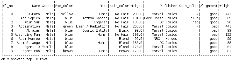

Filtering the Data

Superhero_df.filter(Superhero_df.Gender == 'Male').count() //Male Heros Count

Superhero_df.filter(Superhero_df.Gender == 'Female').count() //Female Heros Count

Grouping the Data

GroupBy is used to group the DataFrame based on the column specified. Here, we are grouping the DataFrame based on the column Race and then with the count function, we can find the count of the particular race.

Race_df = Superhero_df.groupby("Race")\
.count()\
.show()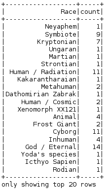

Performing SQL Queries

We can also pass SQL queries directly to any DataFrame, for that we need to create a table from the DataFrame using the registerTempTable method and then use sqlContext.sql() to pass the SQL queries.

Superhero_df.registerTempTable('superhero_table')

sqlContext.sql('select * from superhero_table').show()

sqlContext.sql('select distinct(Eye_color) from superhero_table').show()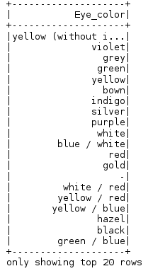

sqlContext.sql('select distinct(Eye_color) from superhero_table').count()

sqlContext.sql('select max(Weight) from superhero_table').show()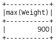

And with this, we come to an end of this PySpark DataFrame Tutorial.

I hope you guys got an idea of what PySpark DataFrame is, why is it used in the industry and its features in this PySpark DataFrame tutorial. Congratulations, you are no longer a newbie to DataFrames.