Introduction to precrec (original) (raw)
The precrec package provides accurate computations of ROC and Precision-Recall curves.
1. Basic functions
The evalmod function calculates ROC and Precision-Recall curves and returns an S3 object.
library(precrec)
# Load a test dataset
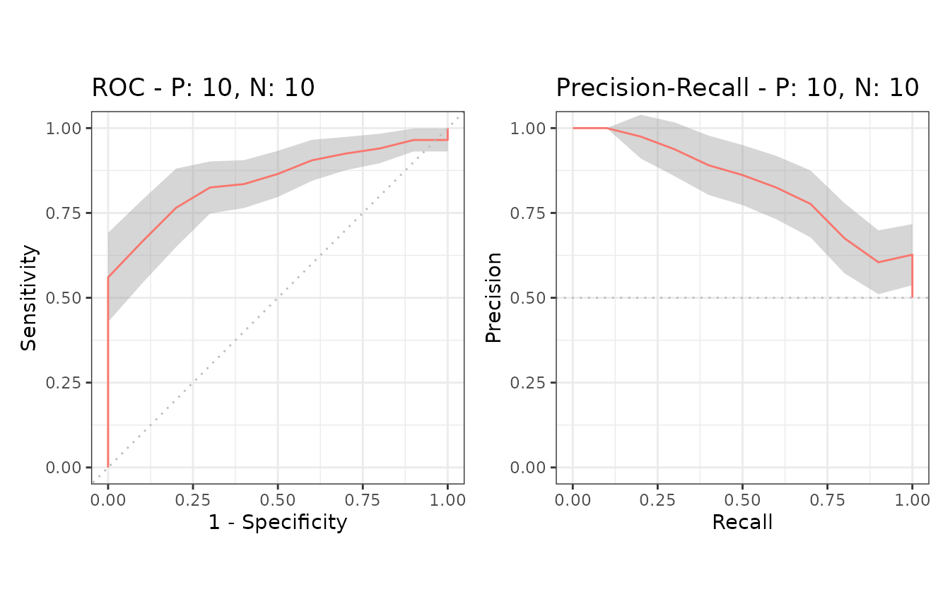
data(P10N10)
# Calculate ROC and Precision-Recall curves
sscurves <- evalmod(scores = P10N10$scores, labels = P10N10$labels)S3 generics
The R language specifies S3 objects and S3 generic functions as part of the most basic object-oriented system in R. The precrecpackage provides nine S3 generics for the S3 object created by theevalmod function.
| S3 generic | Package | Description |
|---|---|---|
| base | Print the calculation results and the summary of the test data | |
| as.data.frame | base | Convert a precrec object to a data frame |
| plot | graphics | Plot performance evaluation measures |
| autoplot | ggplot2 | Plot performance evaluation measures with ggplot2 |
| fortify | ggplot2 | Prepare a data frame for ggplot2 |
| auc | precrec | Make a data frame with AUC scores |
| part | precrec | Set partial curves and calculate AUC scores |
| pauc | precrec | Make a data frame with pAUC scores |
| auc_ci | precrec | Calculate confidence intervals of AUC scores |
Example of the plot function
The plot function outputs ROC and Precision-Recall curves
# Show ROC and Precision-Recall plots
plot(sscurves)
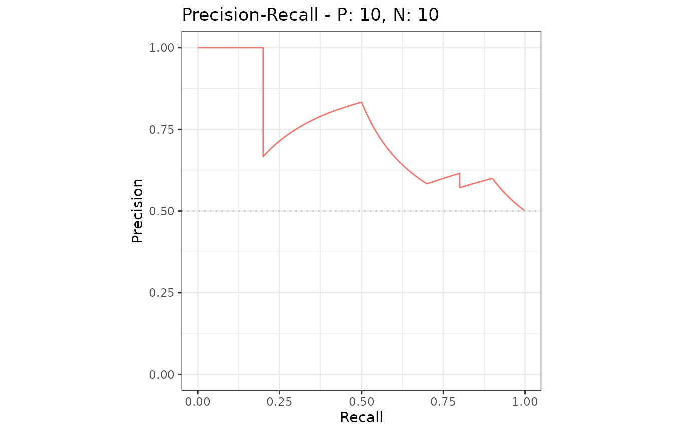
# Show a Precision-Recall plot
plot(sscurves, "PRC")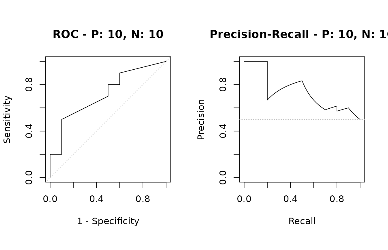

Example of the autoplot function
The autoplot function outputs ROC and Precision-Recall curves by using the ggplot2 package.
# The ggplot2 package is required
library(ggplot2)

# Show ROC and Precision-Recall plots
autoplot(sscurves)

# Show a Precision-Recall plot
autoplot(sscurves, "PRC")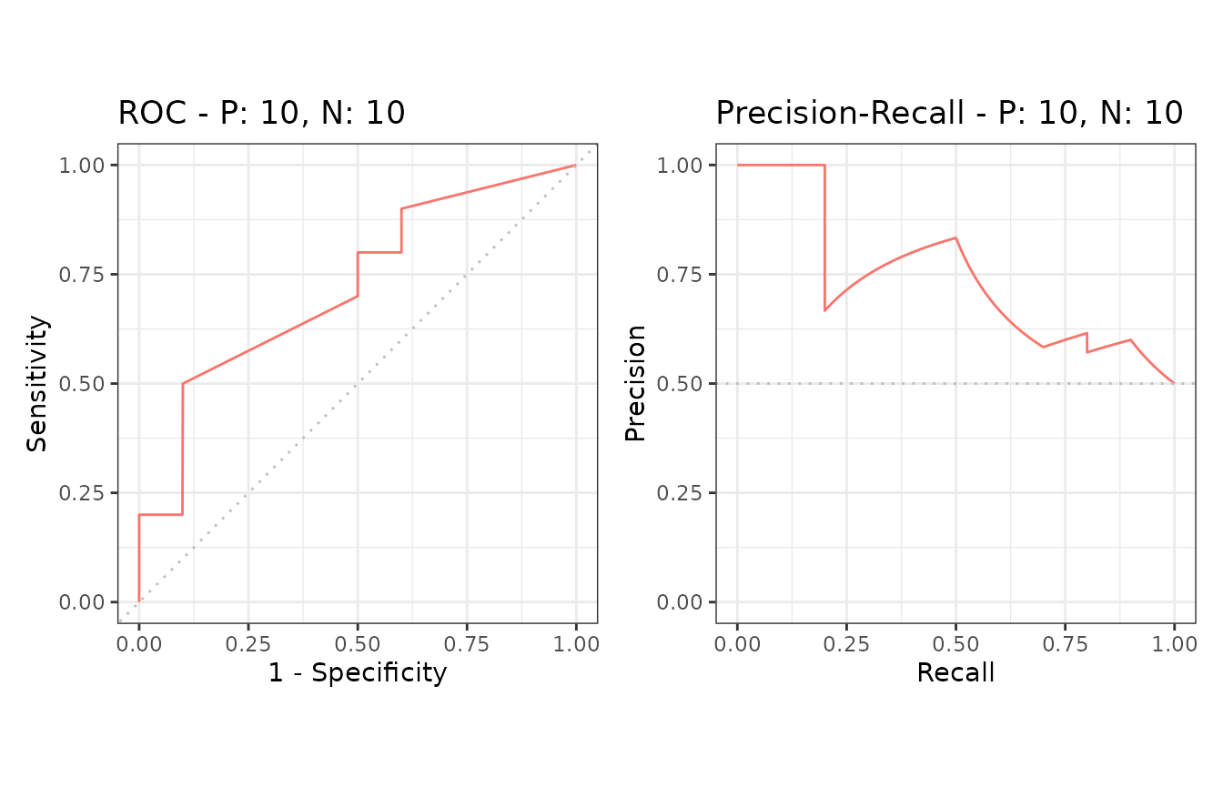
Reduced supporting points make the plotting speed faster for large data sets.
# 5 data sets with 50000 positives and 50000 negatives
samp1 <- create_sim_samples(5, 50000, 50000)

# Calculate curves
eval1 <- evalmod(scores = samp1$scores, labels = samp1$labels)

# Reduced supporting points
system.time(autoplot(eval1))

# Full supporting points
system.time(autoplot(eval1, reduce_points = FALSE))
## user system elapsed
## 0.036 0.003 0.039
## user system elapsed
## 0.280 0.016 0.296Example of the auc function
The auc function outputs a data frame with the AUC (Area Under the Curve) scores.
# Get a data frame with AUC scores
aucs <- auc(sscurves)

# Use knitr::kable to display the result in a table format
knitr::kable(aucs)| modnames | dsids | curvetypes | aucs |
|---|---|---|---|
| m1 | 1 | ROC | 0.7200000 |
| m1 | 1 | PRC | 0.7397716 |
# Get AUCs of Precision-Recall
aucs_prc <- subset(aucs, curvetypes == "PRC")
knitr::kable(aucs_prc)| modnames | dsids | curvetypes | aucs | |
|---|---|---|---|---|
| 2 | m1 | 1 | PRC | 0.7397716 |
Example of the as.data.frame function
The as.data.frame function converts a precrec object to a data frame.
# Convert sscurves to a data frame
sscurves.df <- as.data.frame(sscurves)

# Use knitr::kable to display the result in a table format
knitr::kable(head(sscurves.df))| x | y | modname | dsid | type |
|---|---|---|---|---|
| 0.000 | 0.0 | m1 | 1 | ROC |
| 0.000 | 0.1 | m1 | 1 | ROC |
| 0.000 | 0.2 | m1 | 1 | ROC |
| 0.001 | 0.2 | m1 | 1 | ROC |
| 0.002 | 0.2 | m1 | 1 | ROC |
| 0.003 | 0.2 | m1 | 1 | ROC |
2. Data preparation
The precrec package provides four functions for data preparation.
| Function | Description |
|---|---|
| join_scores | Join scores of multiple models into a list |
| join_labels | Join observed labels of multiple test datasets into a list |
| mmdata | Reformat input data for performance evaluation calculation |
| create_sim_samples | Create random samples for simulations |
Example of the join_scores function
The join_scores function combines multiple score datasets.
s1 <- c(1, 2, 3, 4)
s2 <- c(5, 6, 7, 8)
s3 <- matrix(1:8, 4, 2)

# Join two score vectors
scores1 <- join_scores(s1, s2)

# Join two vectors and a matrix
scores2 <- join_scores(s1, s2, s3)
Example of the join_labels function
The join_labels function combines multiple score datasets.
l1 <- c(1, 0, 1, 1)
l2 <- c(1, 0, 1, 1)
l3 <- c(1, 0, 1, 0)

# Join two label vectors
labels1 <- join_labels(l1, l2)
labels2 <- join_labels(l1, l3)
Example of the mmdata function
The mmdata function makes an input dataset for theevalmod function.
# Create an input dataset with two score vectors and one label vector
msmdat <- mmdata(scores1, labels1)

# Specify dataset IDs
smmdat <- mmdata(scores1, labels2, dsids = c(1, 2))

# Specify model names and dataset IDs
mmmdat <- mmdata(scores1, labels2,
  modnames = c("mod1", "mod2"),
  dsids = c(1, 2)
)
Example of the create_sim_samples function
The create_sim_samples function is useful to make a random sample dataset with different performance levels.
| Level name | Description |
|---|---|
| random | Random |
| poor_er | Poor early retrieval |
| good_er | Good early retrieval |
| excel | Excellent |
| perf | Perfect |
| all | All of the above |
# A dataset with 10 positives and 10 negatives for the random performance level
samps1 <- create_sim_samples(1, 10, 10, "random")

#  A dataset for five different performance levels
samps2 <- create_sim_samples(1, 10, 10, "all")

# A dataset with 20 samples for the good early retrieval performance level
samps3 <- create_sim_samples(20, 10, 10, "good_er")

# A dataset with 20 samples for five different performance levels
samps4 <- create_sim_samples(20, 10, 10, "all")
3. Multiple models
The evalmod function calculate performance evaluation for multiple models when multiple model names are specified with themmdata or the evalmod function.
Data preparation
There are several ways to create a dataset with themmdata function for multiple models.
# Use a list with multiple score vectors and a list with a single label vector
msmdat1 <- mmdata(scores1, labels1)

# Explicitly specify model names
msmdat2 <- mmdata(scores1, labels1, modnames = c("mod1", "mod2"))

# Use a sample dataset created by the create_sim_samples function
msmdat3 <- mmdata(samps2[["scores"]], samps2[["labels"]],
  modnames = samps2[["modnames"]]
)
ROC and Precision-Recall calculations
The evalmod function automatically detects multiple models.
# Calculate ROC and Precision-Recall curves for multiple models
mscurves <- evalmod(msmdat3)
S3 generics
All the S3 generics are effective for the S3 object generated by this approach.
# Show ROC and Precision-Recall curves with the ggplot2 package
autoplot(mscurves)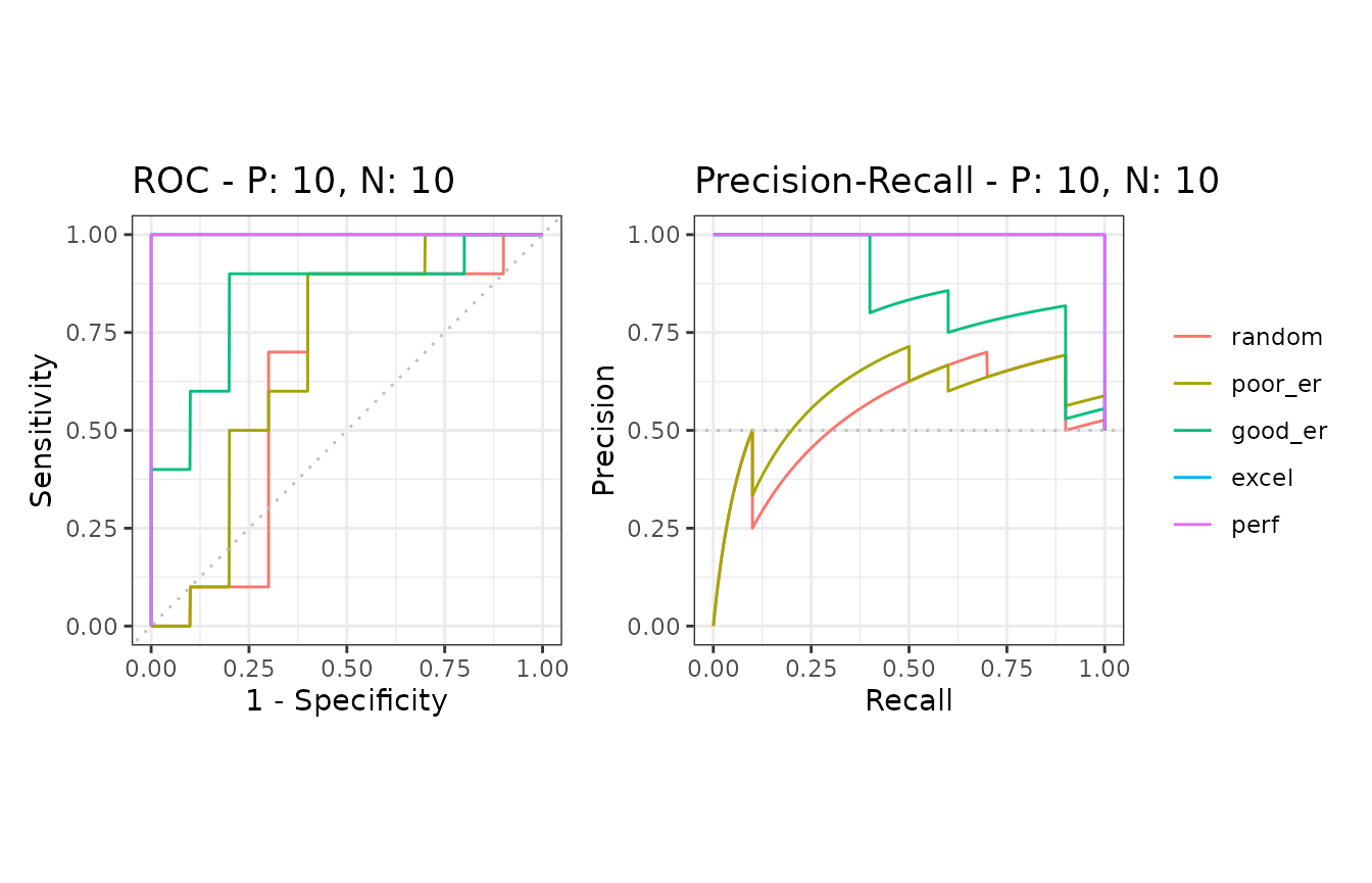
Example of the as.data.frame function
The as.data.frame function also works with this object.
# Convert mscurves to a data frame
mscurves.df <- as.data.frame(mscurves)

# Use knitr::kable to display the result in a table format
knitr::kable(head(mscurves.df))| x | y | modname | dsid | type |
|---|---|---|---|---|
| 0.000 | 0 | random | 1 | ROC |
| 0.001 | 0 | random | 1 | ROC |
| 0.002 | 0 | random | 1 | ROC |
| 0.003 | 0 | random | 1 | ROC |
| 0.004 | 0 | random | 1 | ROC |
| 0.005 | 0 | random | 1 | ROC |
4. Multiple test sets
The evalmod function calculate performance evaluation for multiple test datasets when different test dataset IDs are specified with the mmdata or the evalmod function.
Data preparation
There are several ways to create a dataset with themmdata function for multiple test datasets.
# Specify test dataset IDs names
smmdat1 <- mmdata(scores1, labels2, dsids = c(1, 2))

# Use a sample dataset created by the create_sim_samples function
smmdat2 <- mmdata(samps3[["scores"]], samps3[["labels"]],
  dsids = samps3[["dsids"]]
)
ROC and Precision-Recall calculations
The evalmod function automatically detects multiple test datasets.
# Calculate curves for multiple test datasets and keep all the curves
smcurves <- evalmod(smmdat2, raw_curves = TRUE)
S3 generics
All the S3 generics are effective for the S3 object generated by this approach.
# Show an average Precision-Recall curve with the 95% confidence bounds
autoplot(smcurves, "PRC", show_cb = TRUE)
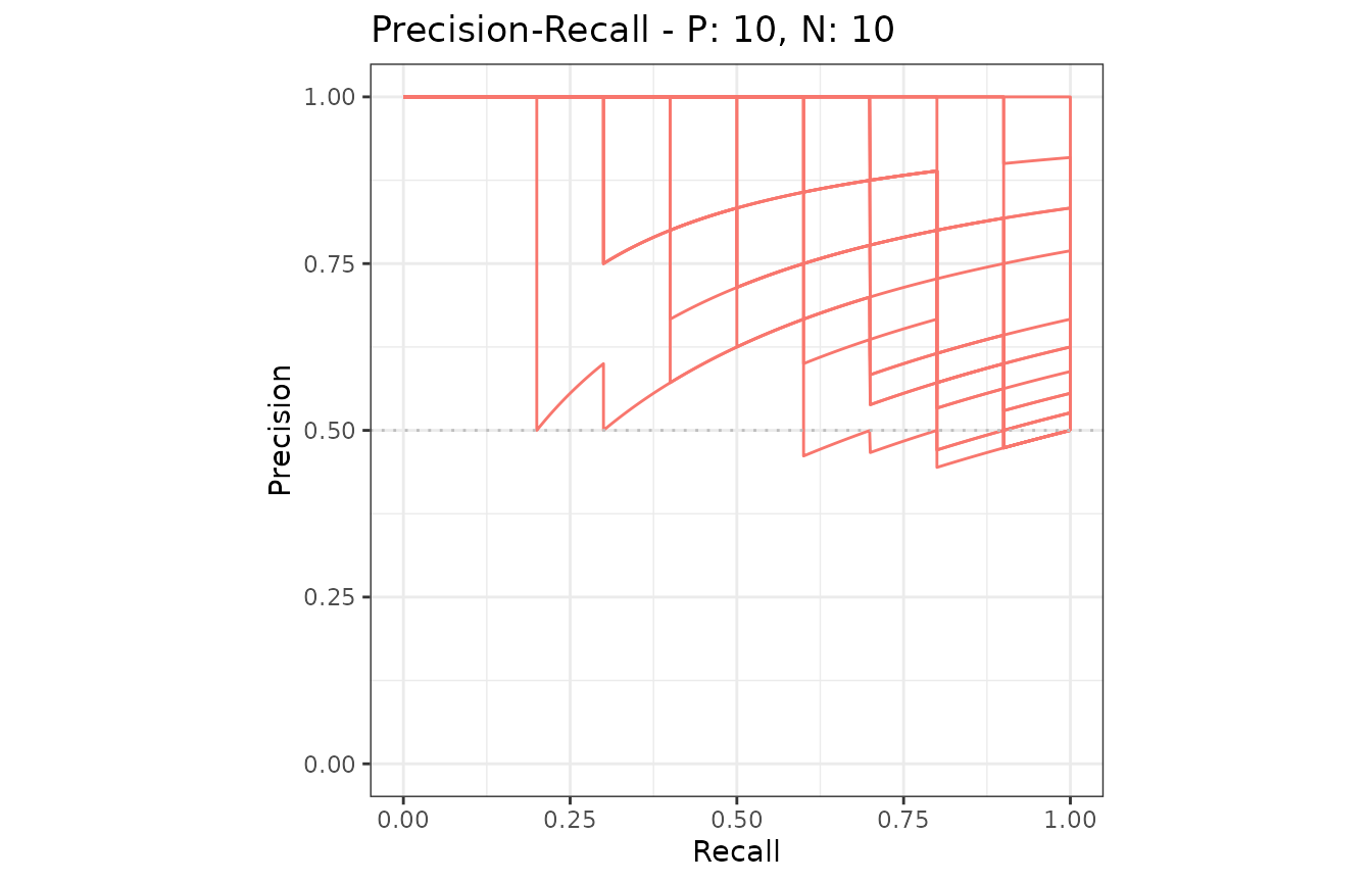
# Show raw Precision-Recall curves
autoplot(smcurves, "PRC", show_cb = FALSE)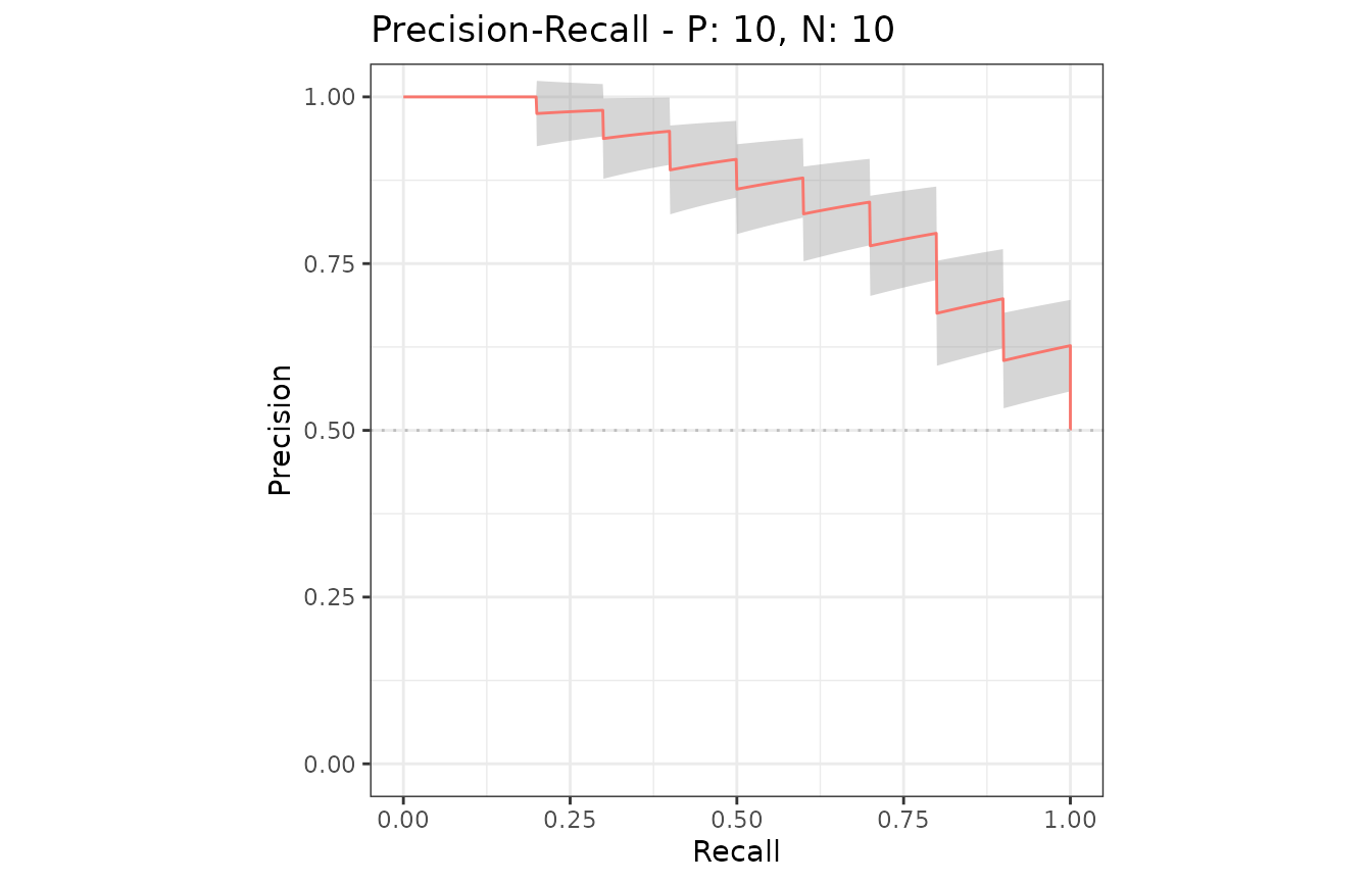
Example of the as.data.frame function
The as.data.frame function also works with this object.
# Convert smcurves to a data frame
smcurves.df <- as.data.frame(smcurves)

# Use knitr::kable to display the result in a table format
knitr::kable(head(smcurves.df))| x | y | modname | dsid | type |
|---|---|---|---|---|
| 0 | 0.0 | m1 | 1 | ROC |
| 0 | 0.1 | m1 | 1 | ROC |
| 0 | 0.2 | m1 | 1 | ROC |
| 0 | 0.3 | m1 | 1 | ROC |
| 0 | 0.4 | m1 | 1 | ROC |
| 0 | 0.5 | m1 | 1 | ROC |
5. Multiple models and multiple test sets
The evalmod function calculates performance evaluation for multiple models and multiple test datasets when different model names and test dataset IDs are specified with the mmdata or the evalmod function.
Data preparation
There are several ways to create a dataset with themmdata function for multiple models and multiple datasets.
# Specify model names and test dataset IDs names
mmmdat1 <- mmdata(scores1, labels2,
  modnames = c("mod1", "mod2"),
  dsids = c(1, 2)
)

# Use a sample dataset created by the create_sim_samples function
mmmdat2 <- mmdata(samps4[["scores"]], samps4[["labels"]],
  modnames = samps4[["modnames"]], dsids = samps4[["dsids"]]
)
ROC and Precision-Recall calculations
The evalmod function automatically detects multiple models and multiple test datasets.
# Calculate curves for multiple models and multiple test datasets
mmcurves <- evalmod(mmmdat2)
S3 generics
All the S3 generics are effective for the S3 object generated by this approach.
# Show average Precision-Recall curves
autoplot(mmcurves, "PRC")

# Show average Precision-Recall curves with the 95% confidence bounds
autoplot(mmcurves, "PRC", show_cb = TRUE)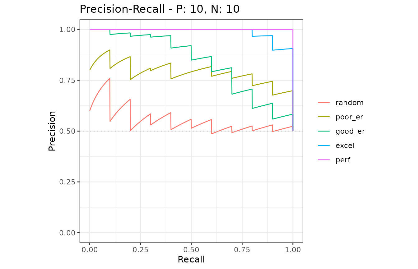
Example of the as.data.frame function
The as.data.frame function also works with this object.
# Convert smcurves to a data frame
mmcurves.df <- as.data.frame(mmcurves)

# Use knitr::kable to display the result in a table format
knitr::kable(head(mmcurves.df))| x | y | ymin | ymax | modname | type |
|---|---|---|---|---|---|
| 0.000 | 0.00 | 0.0000000 | 0.0000000 | random | ROC |
| 0.000 | 0.11 | 0.0551136 | 0.1648864 | random | ROC |
| 0.001 | 0.11 | 0.0551136 | 0.1648864 | random | ROC |
| 0.002 | 0.11 | 0.0551136 | 0.1648864 | random | ROC |
| 0.003 | 0.11 | 0.0551136 | 0.1648864 | random | ROC |
| 0.004 | 0.11 | 0.0551136 | 0.1648864 | random | ROC |
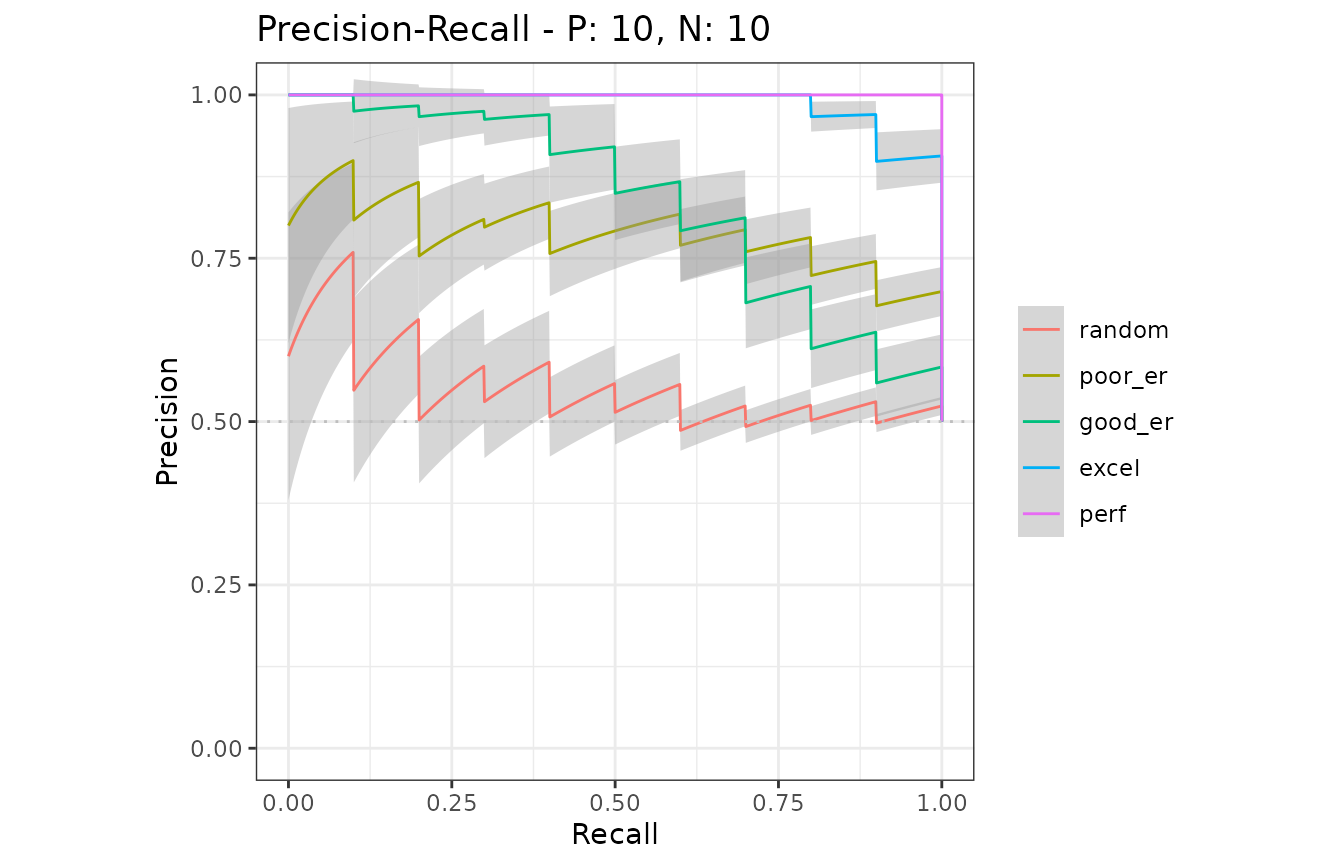
6. Confidence interval bands
The evalmod function automatically calculates confidence bands when a model contains multiple test sets in provided dataset. Confidence intervals are calculated for additional supporting points, which are specified by the ‘x_bins’ option of the evalmodfunction.
Example of confidence bands when x_bins is 2
The dataset smmdat2 contains 20 samples for a single model/classifier.
# Show all curves
smcurves_all <- evalmod(smmdat2, raw_curves = TRUE)
autoplot(smcurves_all)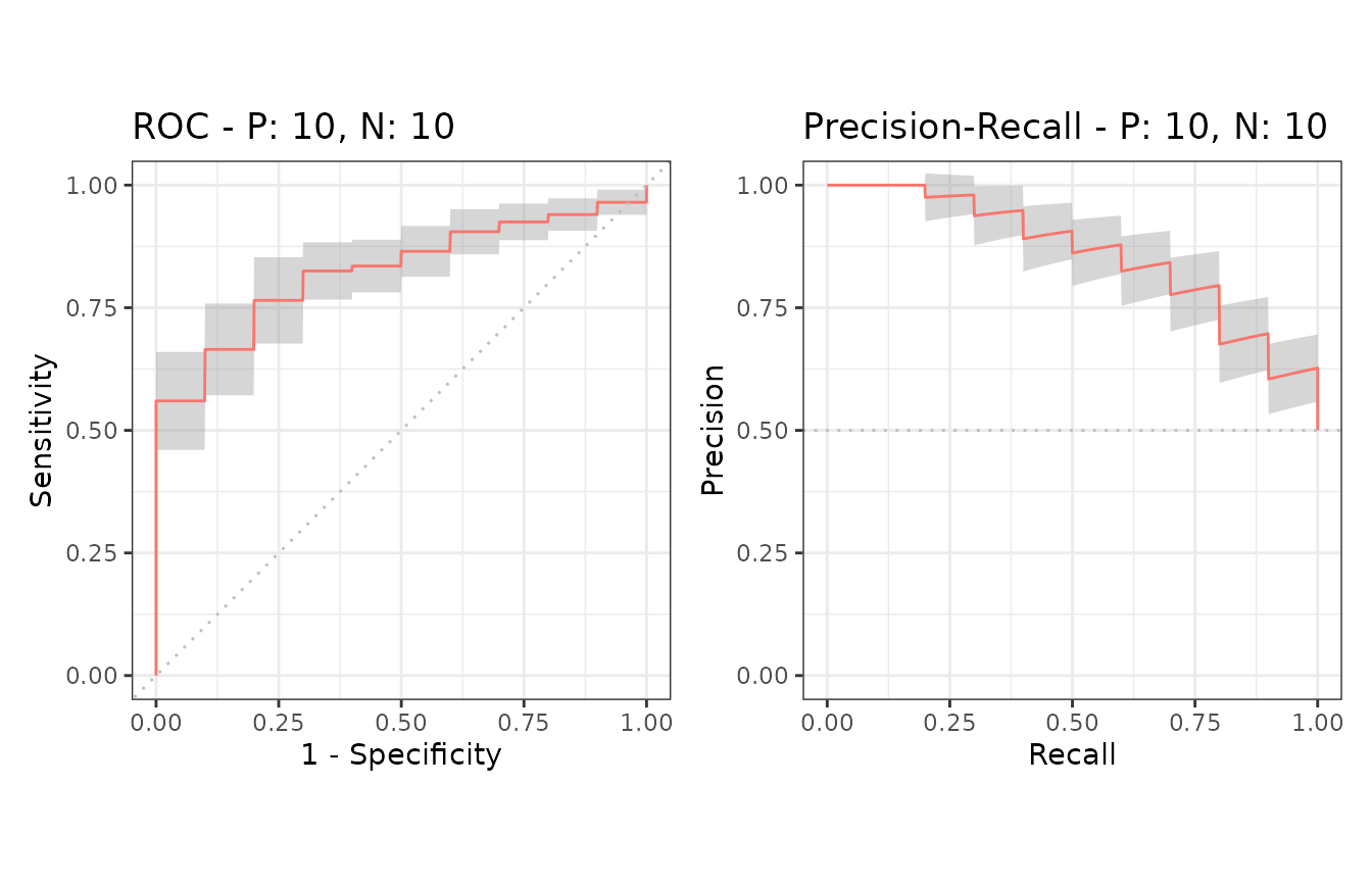
Additional supporting points are calculated forx = (0, 0.5, 1.0) when x_bins is set to 2.
# x_bins: 2
smcurves_xb2 <- evalmod(smmdat2, x_bins = 2)
autoplot(smcurves_xb2)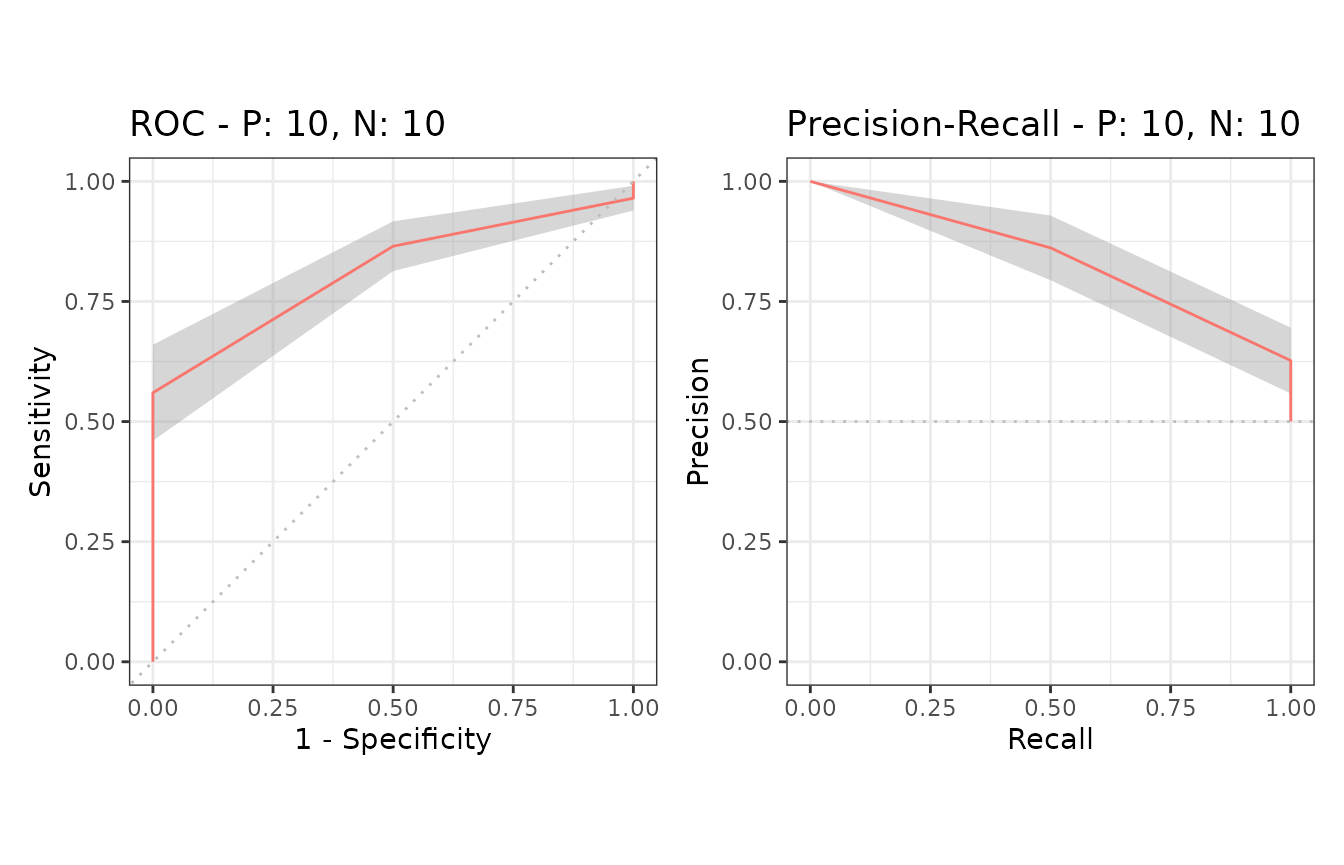
Example of confidence bands when x_bins is 10
Additional supporting points are calculated forx = (0, 0.1, 0.2, 0.3, 0.4, 0.5, 0.6, 0.7, 0.8, 0.9, 1.0)when x_bins is set to 10.
# x_bins: 10
smcurves_xb10 <- evalmod(smmdat2, x_bins = 10)
autoplot(smcurves_xb10)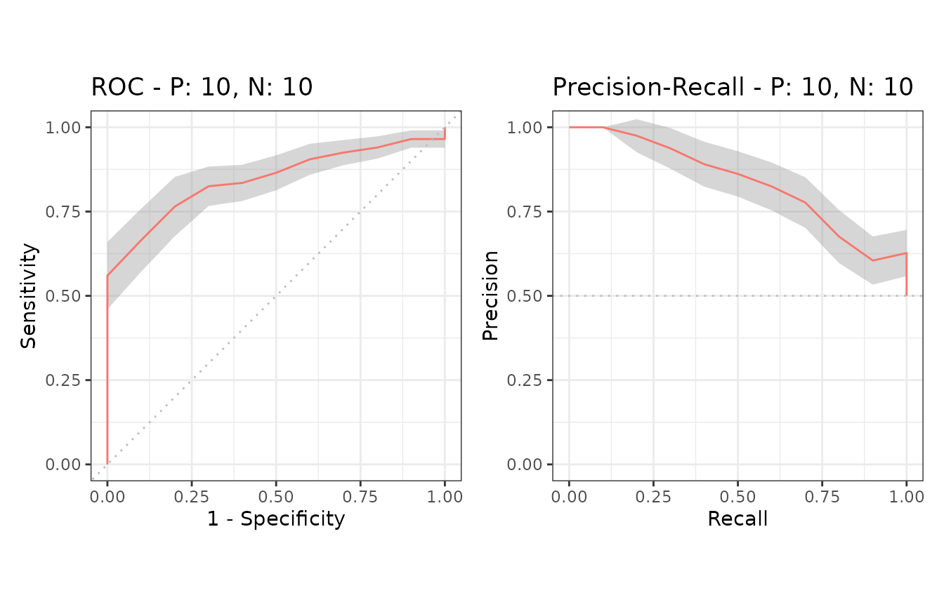
Example of the alpha value
The evalmod function accepts the cb_alphaoption to specify the alpha value of the point-wise confidence bounds calculation. For instance, 95% confidence bands are calculated whencb_alpha is 0.05.
# cb_alpha: 0.1 for 90% confidence band
smcurves_cb1 <- evalmod(smmdat2, x_bins = 10, cb_alpha = 0.1)
autoplot(smcurves_cb1)

# cb_alpha: 0.01 for 99% confidence band
smcurves_cb2 <- evalmod(smmdat2, x_bins = 10, cb_alpha = 0.01)
autoplot(smcurves_cb2)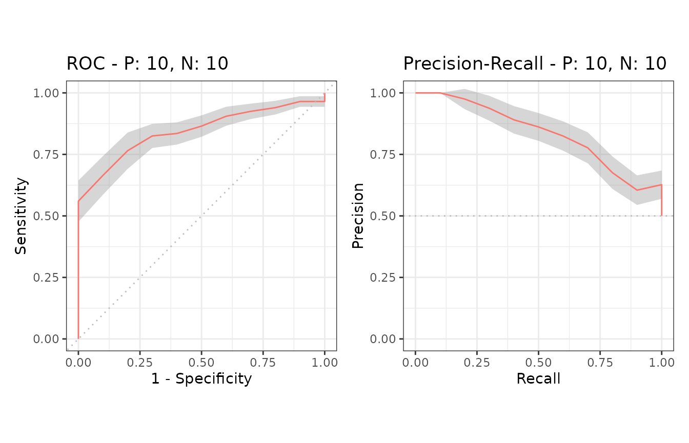
7. Cross validation
The format_nfold function takes a data frame with scores, label and n-fold columns and convert it to a list forevalmod and mmdata.
Example of a data frame with 5-fold data
# Load data
data(M2N50F5)

# Use knitr::kable to display the result in a table format
knitr::kable(head(M2N50F5))| score1 | score2 | label | fold |
|---|---|---|---|
| 2.0606025 | 1.0689227 | pos | 1 |
| 0.3066092 | 0.1745491 | pos | 3 |
| 1.5597733 | -1.5666375 | pos | 1 |
| -0.6044989 | 1.1572727 | pos | 3 |
| -0.2229031 | 0.6070042 | pos | 5 |
| -0.7679551 | -1.7908147 | pos | 5 |
Example of the format_nfold function with 5-fold datasets
# Convert data frame to list
nfold_list1 <- format_nfold(
  nfold_df = M2N50F5, score_cols = c(1, 2),
  lab_col = 3, fold_col = 4
)

# Use column names
nfold_list2 <- format_nfold(
  nfold_df = M2N50F5,
  score_cols = c("score1", "score2"),
  lab_col = "label", fold_col = "fold"
)

# Use the result for evalmod
cvcurves <- evalmod(
  scores = nfold_list2$scores, labels = nfold_list2$labels,
  modnames = rep(c("m1", "m2"), each = 5),
  dsids = rep(1:5, 2)
)
autoplot(cvcurves)
evalmod and mmdata with cross validation datasets
Both evalmod and mmdata function can directly take the arguments of the format_nfoldfunction.
Example of evalmod and mmdata with 5-fold data
# mmdata
cvcurves2 <- mmdata(
  nfold_df = M2N50F5, score_cols = c(1, 2),
  lab_col = 3, fold_col = 4,
  modnames = c("m1", "m2"), dsids = 1:5
)

# evalmod
cvcurves3 <- evalmod(
  nfold_df = M2N50F5, score_cols = c(1, 2),
  lab_col = 3, fold_col = 4,
  modnames = c("m1", "m2"), dsids = 1:5
)
autoplot(cvcurves3)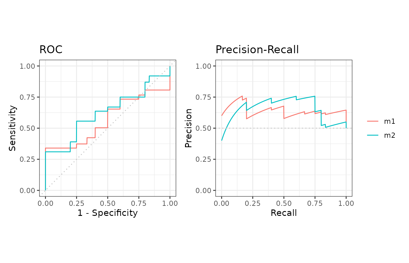
8. Basic performance measures
The evalmod function also calculates basic evaluation measures - error, accuracy, specificity, sensitivity, and precision.
| Measure | Description |
|---|---|
| error | Error rate |
| accuracy | Accuracy |
| specificity | Specificity, TNR, 1 - FPR |
| sensitivity | Sensitivity, TPR, Recall |
| precision | Precision, PPV |
| mcc | Matthews correlation coefficient |
| fscore | F-score |
Basic measure calculations
The mode = "basic" option makes the evalmodfunction calculate the basic evaluation measures instead of performing ROC and Precision-Recall calculations.
# Calculate basic evaluation measures
mmpoins <- evalmod(mmmdat2, mode = "basic")
S3 generics
All the S3 generics except for auc, partand pauc are effective for the S3 object generated by this approach.
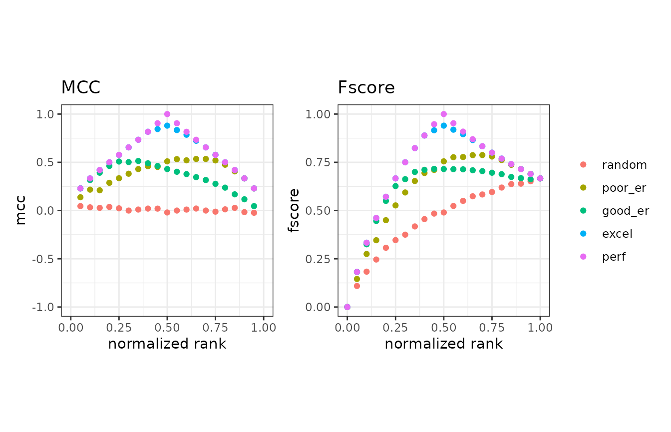
# Show normalized ranks vs. error rate and accuracy
autoplot(mmpoins, c("error", "accuracy"))

# Show normalized ranks vs. specificity, sensitivity, and precision
autoplot(mmpoins, c("specificity", "sensitivity", "precision"))

# Show normalized ranks vs. Matthews correlation coefficient and F-score
autoplot(mmpoins, c("mcc", "fscore"))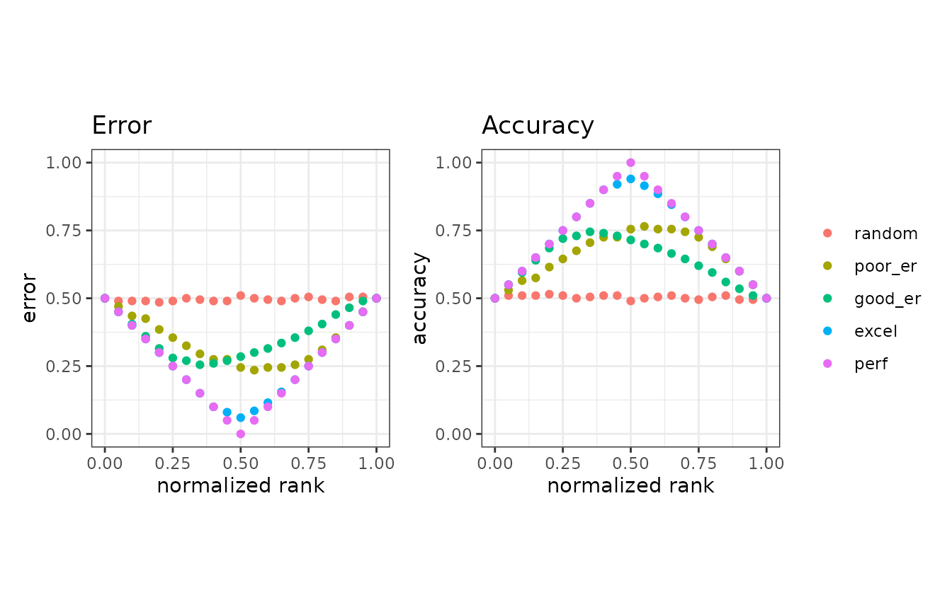
Normalized ranks and predicted scores
In addition to the basic measures, the autoplot function can plot normalized ranks vs. scores and labels.
# Show normalized ranks vs. scores and labels
autoplot(mmpoins, c("score", "label"))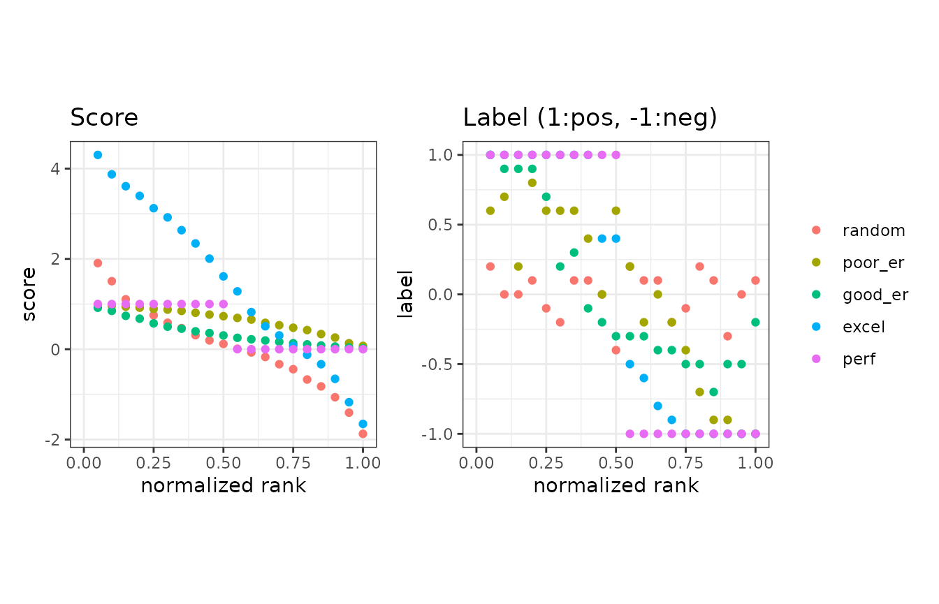
Example of the as.data.frame function
The as.data.frame function also works for the precrec objects of the basic measures.
# Convert mmpoins to a data frame
mmpoins.df <- as.data.frame(mmpoins)

# Use knitr::kable to display the result in a table format
knitr::kable(head(mmpoins.df))| x | y | ymin | ymax | modname | type |
|---|---|---|---|---|---|
| 0.00 | NA | NA | NA | random | score |
| 0.05 | 1.9070654 | 1.7380924 | 2.0760385 | random | score |
| 0.10 | 1.5066177 | 1.3351867 | 1.6780487 | random | score |
| 0.15 | 1.1050874 | 0.9964915 | 1.2136833 | random | score |
| 0.20 | 0.9248578 | 0.8297744 | 1.0199411 | random | score |
| 0.25 | 0.7523308 | 0.6490989 | 0.8555627 | random | score |
9. Partial AUCs
The part function calculates partial AUCs and standardized partial AUCs of both ROC and precision-recall curves. Standardized pAUCs (spAUCs) are standardized to the score range between 0 and 1.
partial AUC calculations
It requires an S3 object produced by the evalmodfunction and uses xlim and ylim to specify the partial area of your choice. The pauc function outputs a data frame with the pAUC scores.
# Calculate ROC and Precision-Recall curves
curves <- evalmod(scores = P10N10$scores, labels = P10N10$labels)

# Calculate partial AUCs
curves.part <- part(curves, xlim = c(0.0, 0.25))

# Retrieve a dataframe of pAUCs
paucs.df <- pauc(curves.part)

# Use knitr::kable to display the result in a table format
knitr::kable(paucs.df)| modnames | dsids | curvetypes | paucs | spaucs |
|---|---|---|---|---|
| m1 | 1 | ROC | 0.1006250 | 0.4025000 |
| m1 | 1 | PRC | 0.2345849 | 0.9383396 |
S3 generics
All the S3 generics are effective for the S3 object generated by this approach.
# Show ROC and Precision-Recall curves
autoplot(curves.part)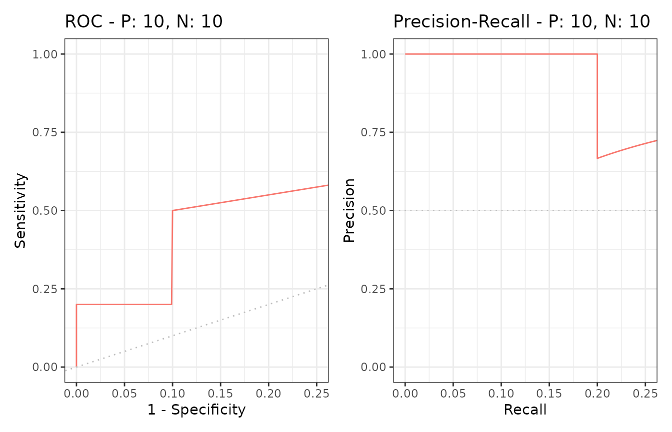
10. Fast AUC (ROC) calculation
The area under the ROC curve can be calculated from the U statistic, which is the test statistic of the Mann–Whitney U test.
AUC calculation with the U statistic
The evalmod function calculates AUCs with the U statistic when mode = ‘aucroc’.
# Calculate AUC (ROC)
aucs <- evalmod(scores = P10N10$scores, labels = P10N10$labels, mode = "aucroc")

# Convert to data.frame
aucs.df <- as.data.frame(aucs)

# Use knitr::kable to display the result in a table format
knitr::kable(aucs.df)| modnames | dsids | aucs | ustats |
|---|---|---|---|
| m1 | 1 | 0.72 | 72 |
11. Confidence intervals of AUCs
The auc_ci function calculates confidence intervals of the calculated ROCs by the evalmod function.
Default CI calculation with normal distribution and alpha=0.05
The auc_ci function calculates CIs for both ROC and precision-recall AUCs. The specified data must contain multiple datasets, such as cross-validation data.
# Calculate CI of AUCs with normal distibution
auc_ci <- auc_ci(smcurves)

# Use knitr::kable to display the result in a table format
knitr::kable(auc_ci)| modnames | curvetypes | mean | error | lower_bound | upper_bound | n |
|---|---|---|---|---|---|---|
| m1 | ROC | 0.8250000 | 0.0503423 | 0.7746577 | 0.8753423 | 20 |
| m1 | PRC | 0.8613514 | 0.0405382 | 0.8208132 | 0.9018896 | 20 |
CI calculation with a different alpha (0.01)
The auc_ci function accepts a different significance level.
# Calculate CI of AUCs with alpha = 0.01
auc_ci_a <- auc_ci(smcurves, alpha = 0.01)

# Use knitr::kable to display the result in a table format
knitr::kable(auc_ci_a)| modnames | curvetypes | mean | error | lower_bound | upper_bound | n |
|---|---|---|---|---|---|---|
| m1 | ROC | 0.8250000 | 0.0661611 | 0.7588389 | 0.8911611 | 20 |
| m1 | PRC | 0.8613514 | 0.0532762 | 0.8080752 | 0.9146276 | 20 |
CI calculation with t-distribution
The auc_ci function accepts either normal or t-distribution for CI calculation.
# Calculate CI of AUCs t-distribution
auc_ci_t <- auc_ci(smcurves, dtype = "t")

# Use knitr::kable to display the result in a table format
knitr::kable(auc_ci_t)| modnames | curvetypes | mean | error | lower_bound | upper_bound | n |
|---|---|---|---|---|---|---|
| m1 | ROC | 0.8250000 | 0.0537600 | 0.7712400 | 0.8787600 | 20 |
| m1 | PRC | 0.8613514 | 0.0432903 | 0.8180611 | 0.9046417 | 20 |
12. Balanced and imbalanced datasets
It is easy to simulate various scenarios, such as balanced vs. imbalanced datasets, by using the evalmod andcreate_sim_samples functions.
Data preparation
# Balanced dataset
samps5 <- create_sim_samples(100, 100, 100, "all")
simmdat1 <- mmdata(samps5[["scores"]], samps5[["labels"]],
modnames = samps5[["modnames"]], dsids = samps5[["dsids"]]
)
# Imbalanced dataset
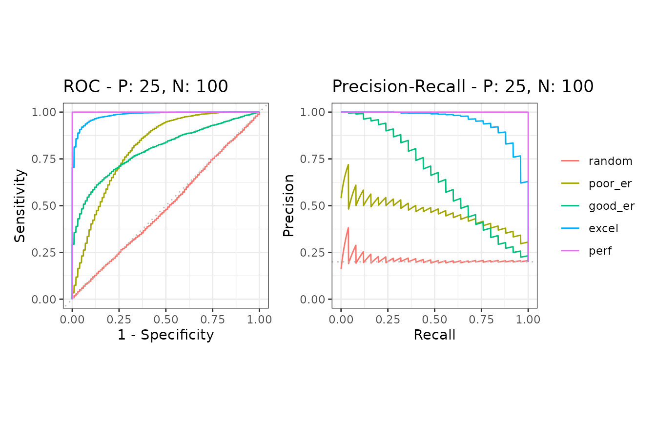
samps6 <- create_sim_samples(100, 25, 100, "all")
simmdat2 <- mmdata(samps6[["scores"]], samps6[["labels"]],
modnames = samps6[["modnames"]], dsids = samps6[["dsids"]]
)ROC and Precision-Recall calculations
The evalmod function automatically detects multiple models and multiple test datasets.
# Balanced dataset
simcurves1 <- evalmod(simmdat1)

# Imbalanced dataset
simcurves2 <- evalmod(simmdat2)
Balanced vs. imbalanced datasets
ROC plots are unchanged between balanced and imbalanced datasets, whereas Precision-Recall plots show a clear difference between them. See our articleor website for potential pitfalls by using ROC plots with imbalanced datasets.
# Balanced dataset
autoplot(simcurves1)

# Imbalanced dataset
autoplot(simcurves2)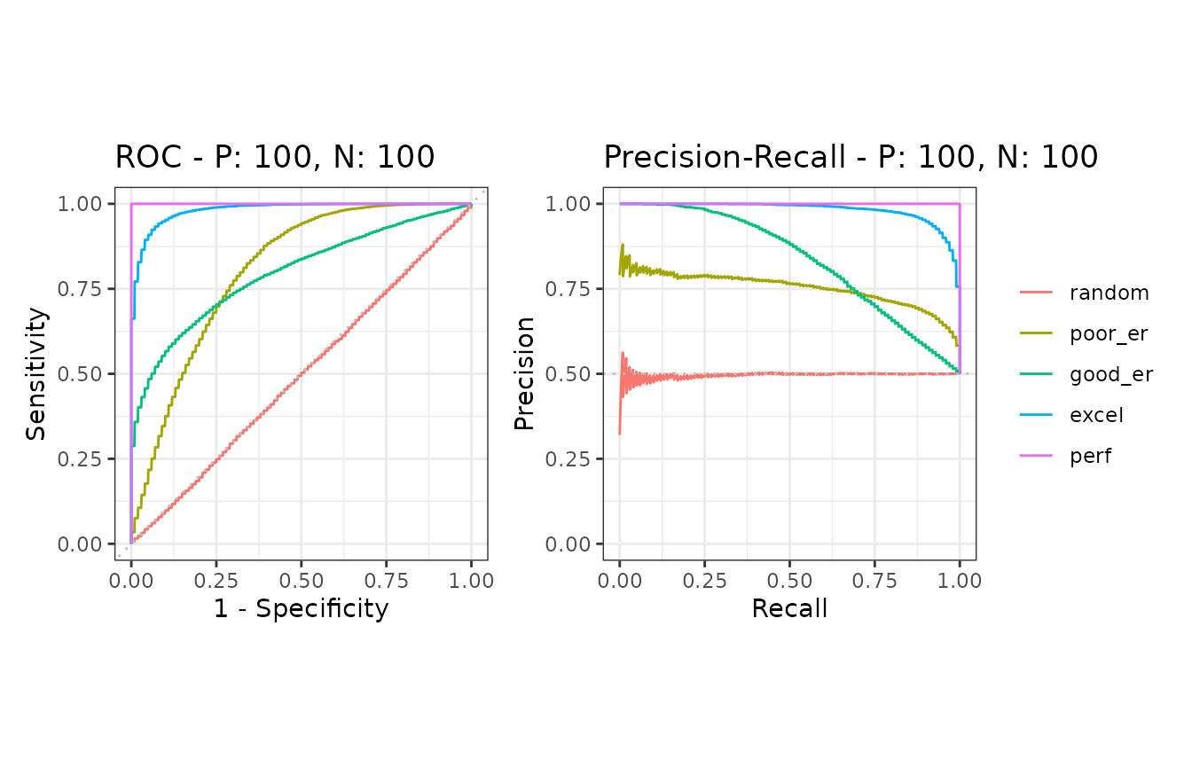
13. Citation
Precrec: fast and accurate precision-recall and ROC curve calculations in R
Takaya Saito; Marc Rehmsmeier
Bioinformatics 2017; 33 (1): 145-147.
doi: 10.1093/bioinformatics/btw570
14. External links
- Classifier evaluation with imbalanced datasets - our web site that contains several pages with useful tips for performance evaluation on binary classifiers.
- The Precision-Recall Plot Is More Informative than the ROC Plot When Evaluating Binary Classifiers on Imbalanced Datasets - our paper that summarized potential pitfalls of ROC plots with imbalanced datasets and advantages of using precision-recall plots instead.