Data Types – Part 1 – Create Your Own Data Types in Power Query (original) (raw)
How can you create your own data types in Excel? Oh yes, you can do it! In this article, we’ll learn how you can create data types in Power Query. Follow the tutorial below.
If you don’t know about data types, we recommend you first watch an introductory video here.
How – to
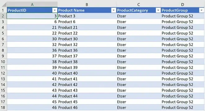
We’ll start with the following tables: the first is the Product table.
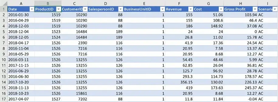
And second is the Sales table.
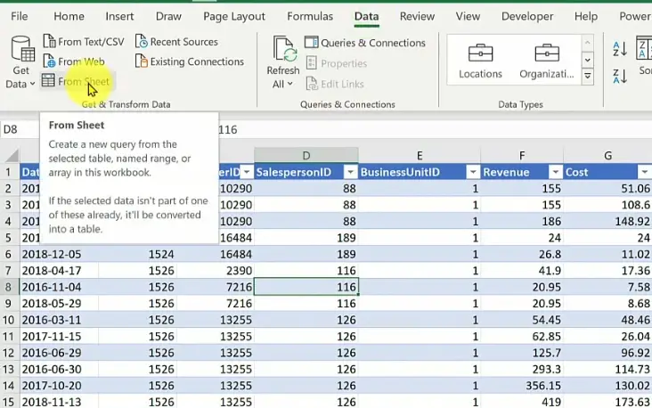
To load to Power Query, select the Sales table and go to Data > From Sheet.
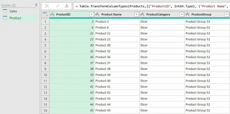
Repeat for the Product table. We now have both tables in Power Query.
Select ProductID column in Sales table and then Home > MergeQueries.
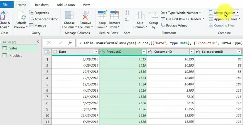
Set column Product table as the second table and select the ProductID column.
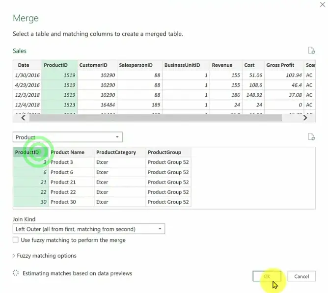
Confirm with OK.
What we’re doing here is we’re actually merging the dimension table the fact table. We would usually never do that, but we’ll demonstrate one useful reason to do it.
Expand the Product name, the Product Category and ProductGroup columns.
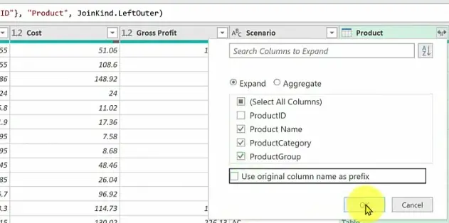
Move the three columns left, right after ProductID.
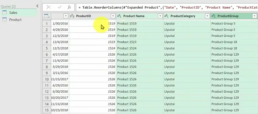
Create the Data Type
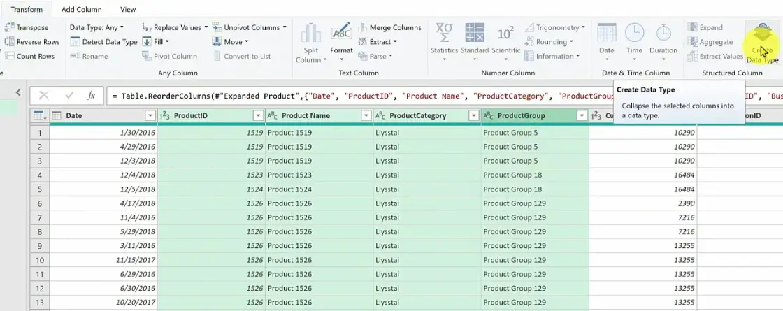
The step you’ve been waiting for! Select the 4 column and then Transform > Create Datatype.
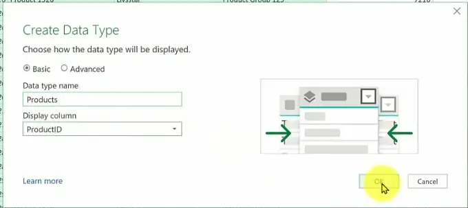
Enter Product as Data type name and ProductsID as Display column. Confirm with OK.
Here’s what will happen: only Products column will remain, the rest will be »inserted« into the Products column.
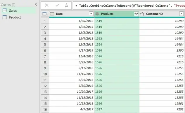
As we see we only the Products column remains. It’s a data type and it also has the expand option.
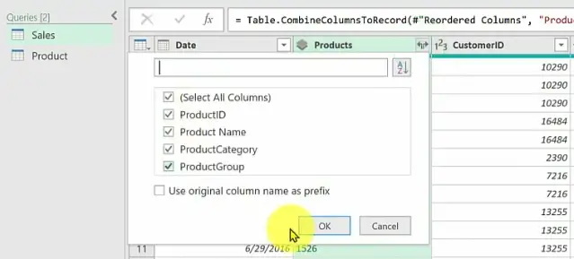
If we open the Expand button, we get the available columns we know. We won’t expand the column so just click Cancel here.
We’ll load the tables into Excel. Select Home > Close and load.
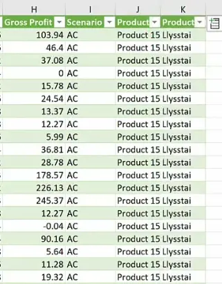
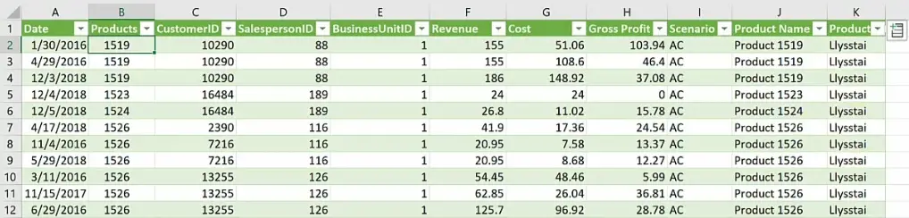
Table we get in Excel looks the same as table before.
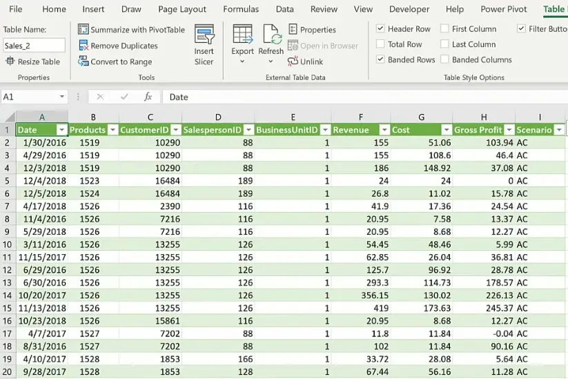
If we select a value in Products column, we get an icon on the right.
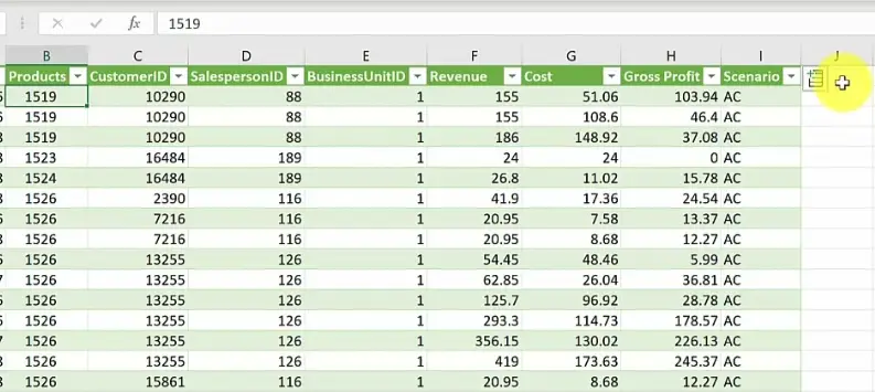
As we click the icon, we see all the columns we saved to this new data type! This means there are multiple columns within Products column.
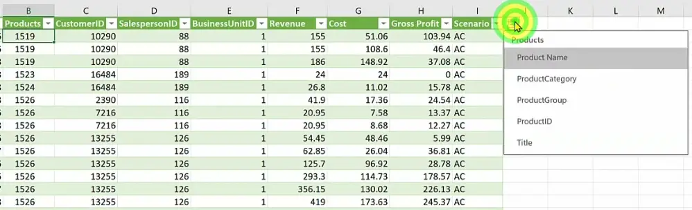
Let’s expand Product Name column.
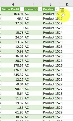
Let’s also expand ProductCategory.
Anytime you need that additional info you simply add it to the table!
We packed the dimension table to the fact table, and we can call up the additional columns anytime we need them. How useful is that!
This concludes our example of how to create your own data types in Power Query. Stay tuned for Part 2, where we’ll show how to do this in Power BI.
Watch the tutorial
Meanwhile, you can also watch the tutorial online on our YouTube channel!
Creating Data Types in Excel – video tutorial
Please leave us a like, comment, and subscribe for more amazing Excel tricks!
Follow us on LinkedIn.
Check out R Academy!