GitHub - rezakj/iCellR: Single (i) Cell R package (iCellR) is an interactive R package to work with high-throughput single cell sequencing technologies (i.e scRNA-seq, scVDJ-seq, scATAC-seq, CITE-Seq and Spatial Transcriptomics (ST)). (original) (raw)

iCellR

iCellR is an interactive R package to work with high-throughput single cell sequencing technologies (i.e scRNA-seq, scVDJ-seq, scATAC-seq, CITE-Seq and Spatial Transcriptomics (ST)).

Maintainer: Alireza Khodadadi-Jamayran

News (April 2021): Use iCellR version 1.6.4 for scATAC-seq and Spatial Transcriptomics (ST). Use the i.score function for scoring (scoring cells based on gene signatures) methods (i.e. tirosh, mean, sum, gsva, ssgsea, zscore and plage).

News (July 2020): See iCellR version 1.5.5 with new cell cycle analysis for G0, G1S, G2M, M, G1M and S phase, Pseudotime Abstract KNetL map (PAK map) and gene-gene correlations. See below for how to.

News (May 2020): see our dimensionality reduction called KNetL map (pronounced like "nettle"). KNetL map is capable of zooming and shows a lot more details compared to tSNE and UMAP.

News (April 2020): see our imputation/coverage correction (CC) and batch alignment (CCCA and CPCA) methods. More databases added for cell type prediction (ImmGen and MCA).

iCellR Viewer (web GUI app): https://compbio.nyumc.org/icellr/

If you are using FlowJo or SeqGeq, they have made plugins for iCellR and other single cell tools: https://www.flowjo.com/exchange/#/ (list of all plugins) and https://www.flowjo.com/exchange/#/plugin/profile?id=34 (iCellR plugin). SeqGeq DE tutorial

For citing iCellR use this PMID: 34353854

iCellR publications: PMID: 35660135 (scRNA-seq/KNetL) PMID: 35180378 (CITE-seq/KNetL), PMID: 34911733 (i.score and cell ranking), PMID: 34963055 (scRNA-seq), PMID 31744829 (scRNA-seq), PMID: 31934613 (bulk RNA-seq from TCGA), PMID: 32550269 (scVDJ-seq), PMID: 34135081, PMID: 33593073, PMID: 34634466, PMID: 35302059, PMID: 34353854

Single (i) Cell R package (iCellR)

How to install iCellR

Install from CRAN

install.packages("iCellR")

Install from github

#library(devtools) #install_github("rezakj/iCellR")

or

#git clone https://github.com/rezakj/iCellR.git #R #install.packages('iCellR/', repos = NULL, type="source")

Download a sample data

Download and unzip a publicly available sample PBMC scRNA-Seq data.

set your working directory

setwd("/your/download/directory")

save the URL as an object

sample.file.url = "https://cf.10xgenomics.com/samples/cell/pbmc3k/pbmc3k_filtered_gene_bc_matrices.tar.gz"

download the file

download.file(url = sample.file.url, destfile = "pbmc3k_filtered_gene_bc_matrices.tar.gz", method = "auto")

unzip the file.

untar("pbmc3k_filtered_gene_bc_matrices.tar.gz")

more data available here:https://genome.med.nyu.edu/results/external/iCellR/

How to use iCellR for analyzing scRNA-seq data

To run a test sample follow these steps:

Go to the R environment load the iCellR package and the PBMC sample data that you downloaded.

library("iCellR") my.data <- load10x("filtered_gene_bc_matrices/hg19/")

This directory includes; barcodes.tsv, genes.tsv/features.tsv and matrix.mtx files

Data could be zipped or unzipped.

if your data is in a csv or tsv format read it like this example

my.data <- read.delim("CITE-Seq_sample_RNA.tsv.gz",header=TRUE)

if your data is in a h5 format read it like this example

library(hdf5r)

data <- load.h5("filtered_feature_bc_matrix.h5")

To see the help page for each function use question mark as:

Aggregate data

Conditions in iCellR are set or shown in the column names of the data and are separated by an underscore "_" sign. Let's say you want to merge multiple datasets (data frames/matrices) into one file and run iCellR in aggregate mode (all samples together). You can do so using "data.aggregation" function. Here’s an example: I divided this sample into four datasets and then aggregated them into one matrix. Here we are assuming you have four samples (e.g. WT,KO,Ctrl,KD). In this way, iCellR will know you have 4 samples for the rest of the analysis (e.g. batch alignment, plots, DE, etc.).

dim(my.data)

[1] 32738 2700

divide your sample into three samples for this example

sample1 <- my.data[1:900] sample2 <- my.data[901:1800] sample3 <- my.data[1801:2300] sample4 <- my.data[2301:2700]

merge all of your samples to make a single aggregated file.

my.data <- data.aggregation(samples = c("sample1","sample2","sample3","sample4"), condition.names = c("WT","KO","Ctrl","KD"))

Check the head of your file.

here is how the head of the first 2 cells in the aggregated file looks like.

head(my.data)[1:2]

WT_AAACATACAACCAC-1 WT_AAACATTGAGCTAC-1

#A1BG 0 0 #A1BG.AS1 0 0 #A1CF 0 0 #A2M 0 0 #A2M.AS1 0 0

as you see the header has the conditions now

Make an object of class iCellR.

my.obj <- make.obj(my.data) my.obj ################################### ,--. ,-----. ,--.,--.,------. --'' .--./ ,---. | || || .--. ' ,--.| | | .-. :| || || '--'.' | |' '--'\ --. | || || | --' -----' ----'--'--'`--' '--' ################################### An object of class iCellR version: 1.6.0 Raw/original data dimentions (rows,columns): 32738,2700 Data conditions in raw data: Ctrl,KD,KO,WT (500,400,900,900) Row names: A1BG,A1BG.AS1,A1CF ... Columns names: WT_AAACATACAACCAC.1,WT_AAACATTGAGCTAC.1,WT_AAACATTGATCAGC.1 ... ################################### QC stats performed:FALSE, PCA performed:FALSE Clustering performed:FALSE, Number of clusters:0 tSNE performed:FALSE, UMAP performed:FALSE, DiffMap performed:FALSE Main data dimensions (rows,columns): 0,0 Normalization factors:,... Imputed data dimensions (rows,columns):0,0 ############## scVDJ-seq ########### VDJ data dimentions (rows,columns):0,0 ############## CITE-seq ############ ADT raw data dimensions (rows,columns):0,0 ADT main data dimensions (rows,columns):0,0 ADT columns names:... ADT row names:... ############## scATAC-seq ############ ATAC raw data dimensions (rows,columns):0,0 ATAC main data dimensions (rows,columns):0,0 ATAC columns names:... ATAC row names:... ############## Spatial ########### Spatial data dimentions (rows,columns):0,0 ########### iCellR object ##########

Perform some QC

my.obj <- qc.stats(my.obj)

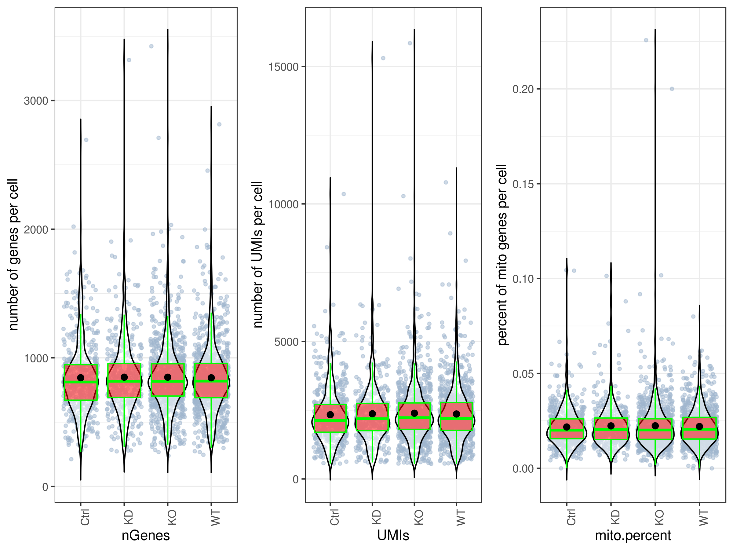
Plot QC

By default all the plotting functions would create interactive html files unless you set this parameter: interactive = FALSE.

plot UMIs, genes and percent mito all at once and in one plot.

you can make them individually as well, see the arguments ?stats.plot.

stats.plot(my.obj, plot.type = "three.in.one", out.name = "UMI-plot", interactive = FALSE, cell.color = "slategray3", cell.size = 1, cell.transparency = 0.5, box.color = "red", box.line.col = "green")

Scatter plots

stats.plot(my.obj, plot.type = "point.mito.umi", out.name = "mito-umi-plot") stats.plot(my.obj, plot.type = "point.gene.umi", out.name = "gene-umi-plot")

Filter cells.

iCellR allows you to filter based on library sizes (UMIs), number of genes per cell, percent mitochondrial content, one or more genes, and cell ids.

my.obj <- cell.filter(my.obj, min.mito = 0, max.mito = 0.05, min.genes = 200, max.genes = 2400, min.umis = 0, max.umis = Inf)

#[1] "cells with min mito ratio of 0 and max mito ratio of 0.05 were filtered." #[1] "cells with min genes of 200 and max genes of 2400 were filtered." #[1] "No UMI number filter" #[1] "No cell filter by provided gene/genes" #[1] "No cell id filter" #[1] "filters_set.txt file has beed generated and includes the filters set for this experiment."

more examples

my.obj <- cell.filter(my.obj, filter.by.gene = c("RPL13","RPL10")) # filter our cell having no counts for these genes

my.obj <- cell.filter(my.obj, filter.by.cell.id = c("WT_AAACATACAACCAC.1")) # filter our cell cell by their cell ids.

chack to see how many cells are left.

dim(my.obj@main.data) #[1] 32738 2637

Down sampling

This step is optional and is for having the same number of cells for each condition.

optional

my.obj <- down.sample(my.obj)

#[1] "From" #[1] "Data conditions: Ctrl,KO,WT (877,877,883)" #[1] "to" #[1] "Data conditions: Ctrl,KO,WT (877,877,877)"

Normalize data

my.obj <- norm.data(my.obj, norm.method = "ranked.glsf", top.rank = 500) # best for scRNA-Seq

more examples

#my.obj <- norm.data(my.obj, norm.method = "ranked.deseq", top.rank = 500) #my.obj <- norm.data(my.obj, norm.method = "deseq") # best for bulk RNA-Seq #my.obj <- norm.data(my.obj, norm.method = "global.glsf") # best for bulk RNA-Seq #my.obj <- norm.data(my.obj, norm.method = "rpm", rpm.factor = 100000) # best for bulk RNA-Seq #my.obj <- norm.data(my.obj, norm.method = "spike.in", spike.in.factors = NULL) #my.obj <- norm.data(my.obj, norm.method = "no.norm") # if the data is already normalized

Perform second QC (optioal)

#my.obj <- qc.stats(my.obj,which.data = "main.data")

#stats.plot(my.obj, # plot.type = "all.in.one", # out.name = "UMI-plot", # interactive = F, # cell.color = "slategray3", # cell.size = 1, # cell.transparency = 0.5, # box.color = "red", # box.line.col = "green", # back.col = "white")

Scale data (optional)

iCellR does not need this step as it scales the data when they need to be scaled on the fly; like for plotting or running PCA. This is because, it is important to use the untransformed data for differential expression analysis to calculate the accurate/true fold changes. If you run this function the scaled data will "not" replace the main data and instead will be saved in different data slot in the object.

my.obj <- data.scale(my.obj)

Gene stats

my.obj <- gene.stats(my.obj, which.data = "main.data")

head(my.obj@gene.data[order(my.obj@gene.data$numberOfCells, decreasing = T),])

genes numberOfCells totalNumberOfCells percentOfCells meanExp

#30303 TMSB4X 2637 2637 100.00000 38.55948 #3633 B2M 2636 2637 99.96208 45.07327 #14403 MALAT1 2636 2637 99.96208 70.95452 #27191 RPL13A 2635 2637 99.92416 32.29009 #27185 RPL10 2632 2637 99.81039 35.43002 #27190 RPL13 2630 2637 99.73455 32.32106

SDs condition

#30303 7.545968e-15 all #3633 2.893940e+01 all #14403 7.996407e+01 all #27191 2.783799e+01 all #27185 2.599067e+01 all #27190 2.661361e+01 all

Make a gene model for clustering

This function will help you find a good number of genes to use for running PCA.

See model plot

make.gene.model(my.obj, my.out.put = "plot", dispersion.limit = 1.5, base.mean.rank = 1500, no.mito.model = T, mark.mito = T, interactive = F, out.name = "gene.model")

Write the gene model data into the object

my.obj <- make.gene.model(my.obj, my.out.put = "data", dispersion.limit = 1.5, base.mean.rank = 1500, no.mito.model = T, mark.mito = T, interactive = F, out.name = "gene.model")

head(my.obj@gene.model)

"ACTB" "ACTG1" "ACTR3" "AES" "AIF1" "ALDOA"

get html plot (optional)

#make.gene.model(my.obj, my.out.put = "plot", # dispersion.limit = 1.5, # base.mean.rank = 1500, # no.mito.model = T, # mark.mito = T, # interactive = T, # out.name = "plot4_gene.model")

To view an the html interactive plot click on this links: Dispersion plot

Perform Principal component analysis (PCA)

Note: skip this step if you plan to do batch correction. For batch correction (sample alignment/harmonization/integration) see the sections; CPCA, CCCA, MNN or anchor alignment.

If you run PCA (run.pca) there would be no batch alignment but if you run CPCA (using iba function) this would perform batch alignment and PCA after batch alignment. Example for batch alignment using iba function:

my.obj <- iba(my.obj,dims = 1:30, k = 10,ba.method = "CPCA", method = "gene.model", gene.list = my.obj@gene.model)

run PCA in case no batch alignment is necessary

my.obj <- run.pca(my.obj, method = "gene.model", gene.list = my.obj@gene.model,data.type = "main")

opt.pcs.plot(my.obj)

2 round PCA (optional)

This is to find top genes in the first 10 PCs and re-run PCA for better clustering.

This is optional and might not be good in some cases

#length(my.obj@gene.model)

683

#my.obj <- find.dim.genes(my.obj, dims = 1:10,top.pos = 20, top.neg = 20) # (optional)

#length(my.obj@gene.model)

211 second round PC

#my.obj <- run.pca(my.obj, method = "gene.model", gene.list = my.obj@gene.model,data.type = "main")

Perform other dimensionality reductions (tSNE, UMAP, KNetL, PHATE, destiny, diffusion maps)

We recommend tSNE, UMAP and KNetL. KNetL is fundamentally more powerful.

tSNE

my.obj <- run.pc.tsne(my.obj, dims = 1:10)

UMAP

my.obj <- run.umap(my.obj, dims = 1:10)

KNetL (for lager than 5000 cell use a zoom of about 400)

Because knetl has a very high resolution it's best to use a dim of 20 (this usually works best for most data)

my.obj <- run.knetl(my.obj, dims = 1:20, zoom = 110) # (Important note!) don't forget to set the zoom in the right range

########################## IMPORTANT DISCLAIMER NOTE ########################### *** KNetL map is very dynamic with zoom and dims! *** *** Therefore it needs to be adjusted! ***

For data with less than 1000 cells use a zoom of about 5-50.

For data with 1000-5000 cells use a zoom of about 50-200.

For data with 5000-10000 cells use a zoom of about 100-300.

For data with 10000-30000 cells use a zoom of about 200-500.

For data with more than 30000 cells use a zoom of about 400-600.

zoom 400 is usually good for big data but adjust for intended resolution.

Lower number for zoom in and higher for zoom out (its reverse).

dims = 1:20 is generally good for most data.

other parameters are best as default.

Just like a microscope, you need to zoom to see the intended amount of details.

Here we use a zoom of 100 or 110 but this might not be ideal for your data.

example: # my.obj <- run.knetl(my.obj, dims = 1:20, zoom = 400)

Because knetl has a very high resolution it's best to use a dim of 20 (this usually works best for most data)

################################################################################### ################################################################################### ################################################################################### ###################################################################################

diffusion map

this requires python packge phate or bioconductor R package destiny

How to install destiny

if (!requireNamespace("BiocManager", quietly = TRUE))

install.packages("BiocManager")

BiocManager::install("destiny")

How to install phate

pip install --user phate

Install phateR version 2.9

wget https://cran.r-project.org/src/contrib/Archive/phateR/phateR_0.2.9.tar.gz

install.packages('phateR/', repos = NULL, type="source")

or

library(devtools)

install_version("phateR", version = "0.2.9", repos = "http://cran.us.r-project.org")

optional

library(destiny)

my.obj <- run.diffusion.map(my.obj, dims = 1:10)

or

library(phateR)

my.obj <- run.diffusion.map(my.obj, dims = 1:10, method = "phate")

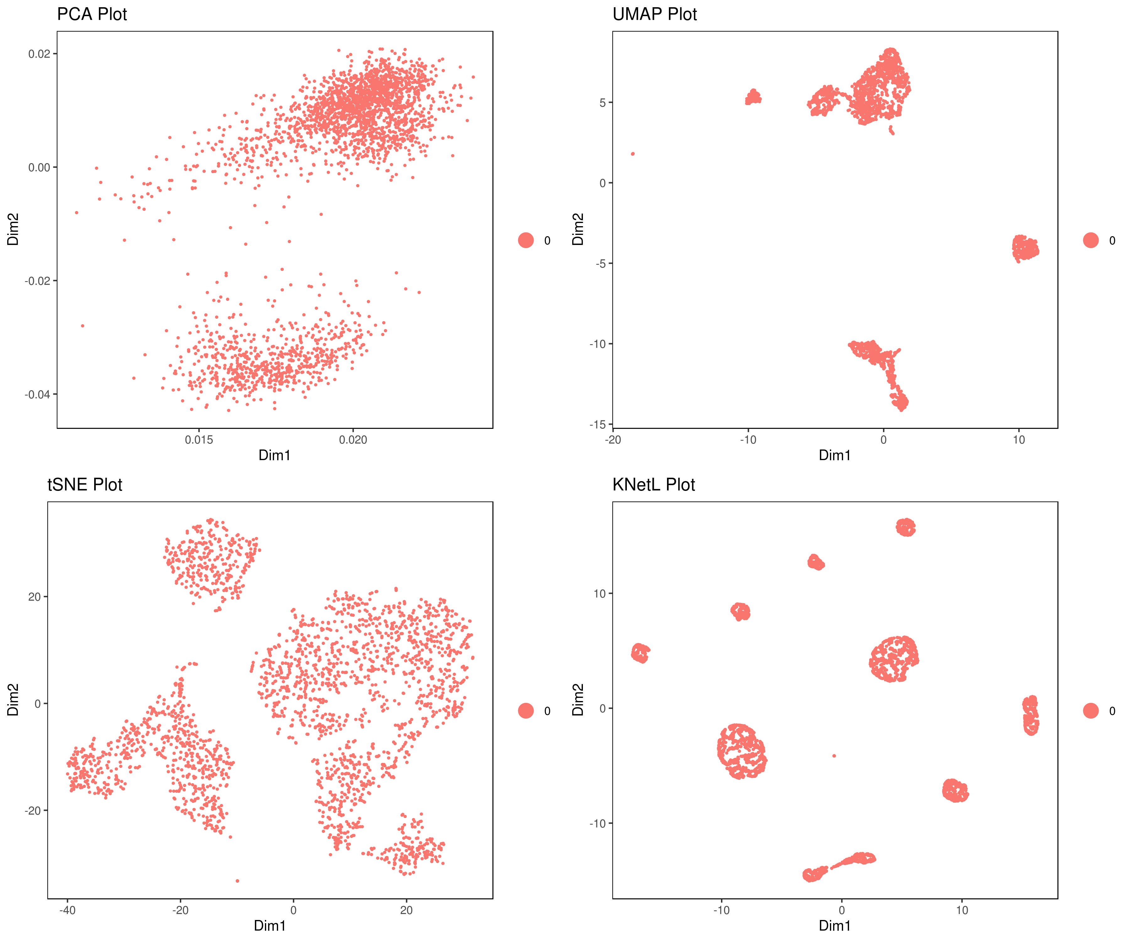
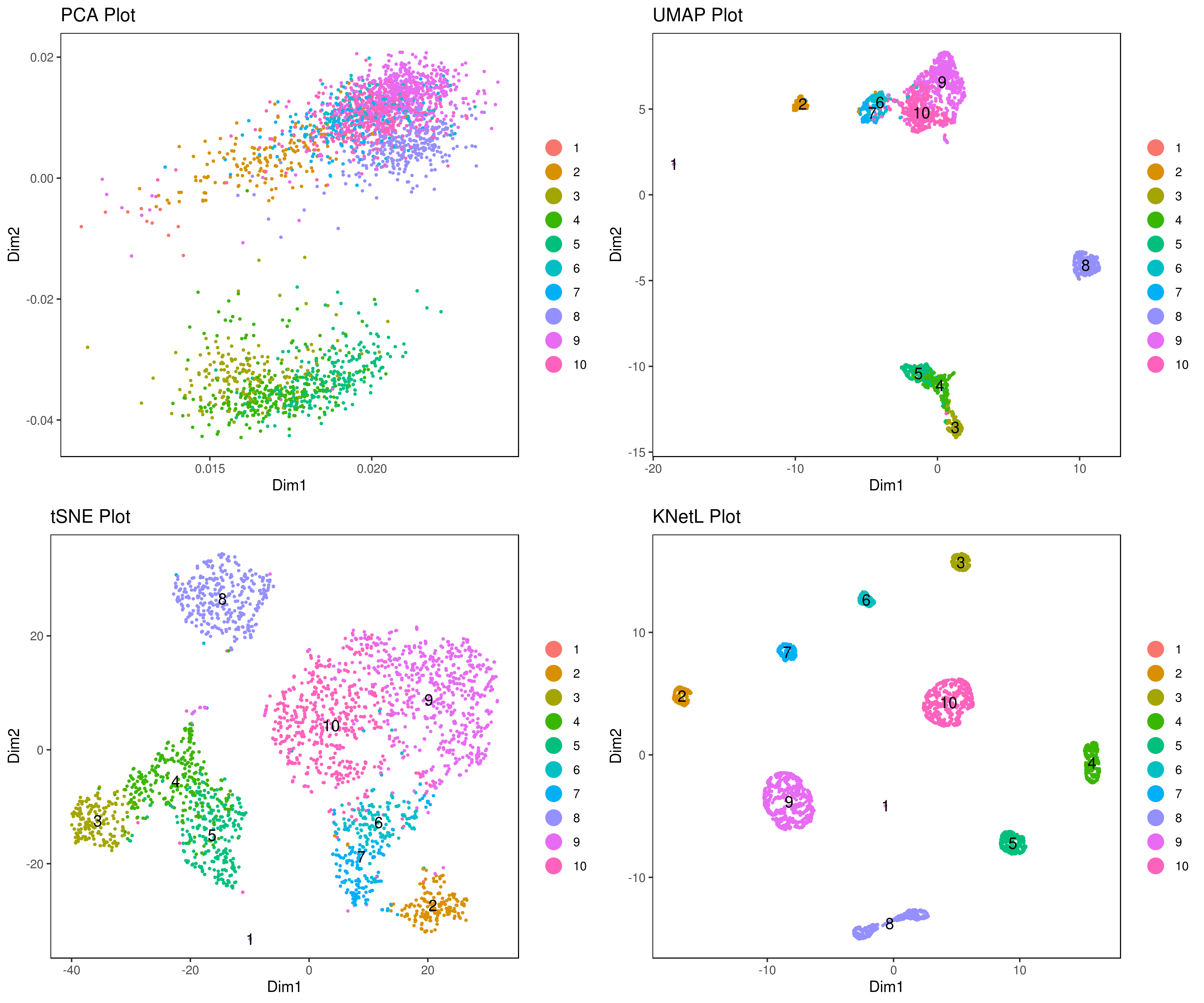
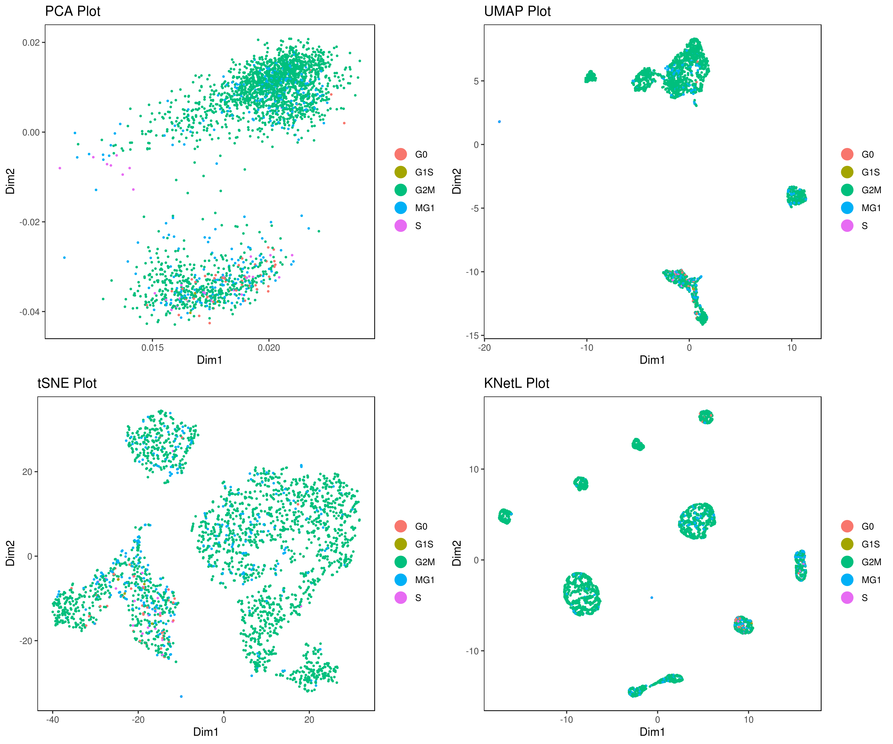
Visualizing the results of dimensionality reductions before clustering (optional)

A= cluster.plot(my.obj,plot.type = "pca",interactive = F) B= cluster.plot(my.obj,plot.type = "umap",interactive = F) C= cluster.plot(my.obj,plot.type = "tsne",interactive = F) D= cluster.plot(my.obj,plot.type = "knetl",interactive = F)

library(gridExtra) grid.arrange(A,B,C,D)

Clustering

We provide three functions to run the clustering method of your choice:

1- iclust (** recommended):

Faster and optimized for iCellR. This function takes PCA, UMAP or tSNE, Destiny (diffusion map), PHATE or KNetL map as input. This function is using Louvain algorithm for clustering a graph made using KNN. Similar to PhenoGraph (Levine et al., Cell, 2015) however instead of Jaccard similarity values we use distance (euclidean by default) values for the weights.

2- run.phenograph:

R implementation of the PhenoGraph algorithm. Rphenograph wrapper (Levine et al., Cell, 2015).

3- run.clustering:

In this function we provide a variety of many other options for you to explore the data with different flavours of clustering and indexing methods. Choose any combinations from the table below.

clustering methods	distance methods	indexing methods
ward.D, ward.D2, single, complete, average, mcquitty, median, centroid, kmeans	euclidean, maximum, manhattan, canberra, binary, minkowski or NULL	kl, ch, hartigan, ccc, scott, marriot, trcovw, tracew, friedman, rubin, cindex, db, silhouette, duda, pseudot2, beale, ratkowsky, ball, ptbiserial, gap, frey, mcclain, gamma, gplus, tau, dunn, hubert, sdindex, dindex, sdbw

This is one of the harder parts of the analysis and sometimes you need to adjust your clustering based on marker genes. This means you might need to merge some clusters, gate (see our cell gating tools) or try different sensitivities to find more or less communities.

clustering based on KNetL

my.obj <- iclust(my.obj, sensitivity = 150, data.type = "knetl")

clustering based on PCA

my.obj <- iclust(my.obj, sensitivity = 150, data.type = "pca", dims=1:10)

play with k to get the clusters right. Usually 150 is good.

more examples

clustering based on PCA

my.obj <- iclust(my.obj,

dist.method = "euclidean",

sensitivity = 100,

dims = 1:10,

data.type = "pca")

or

run.phenograph

my.obj <- run.phenograph(my.obj,k = 100,dims = 1:10)

or

run.clustering

my.obj <- run.clustering(my.obj,

clust.method = "kmeans",

dist.method = "euclidean",

index.method = "silhouette",

max.clust = 25,

min.clust = 2,

dims = 1:10)

If you want to manually set the number of clusters, and not used the predicted optimal number, set the minimum and maximum to the number you want:

#my.obj <- run.clustering(my.obj, # clust.method = "ward.D", # dist.method = "euclidean", # index.method = "ccc", # max.clust = 8, # min.clust = 8, # dims = 1:10)

more examples

#my.obj <- run.clustering(my.obj, # clust.method = "ward.D", # dist.method = "euclidean", # index.method = "kl", # max.clust = 25, # min.clust = 2, # dims = 1:10)

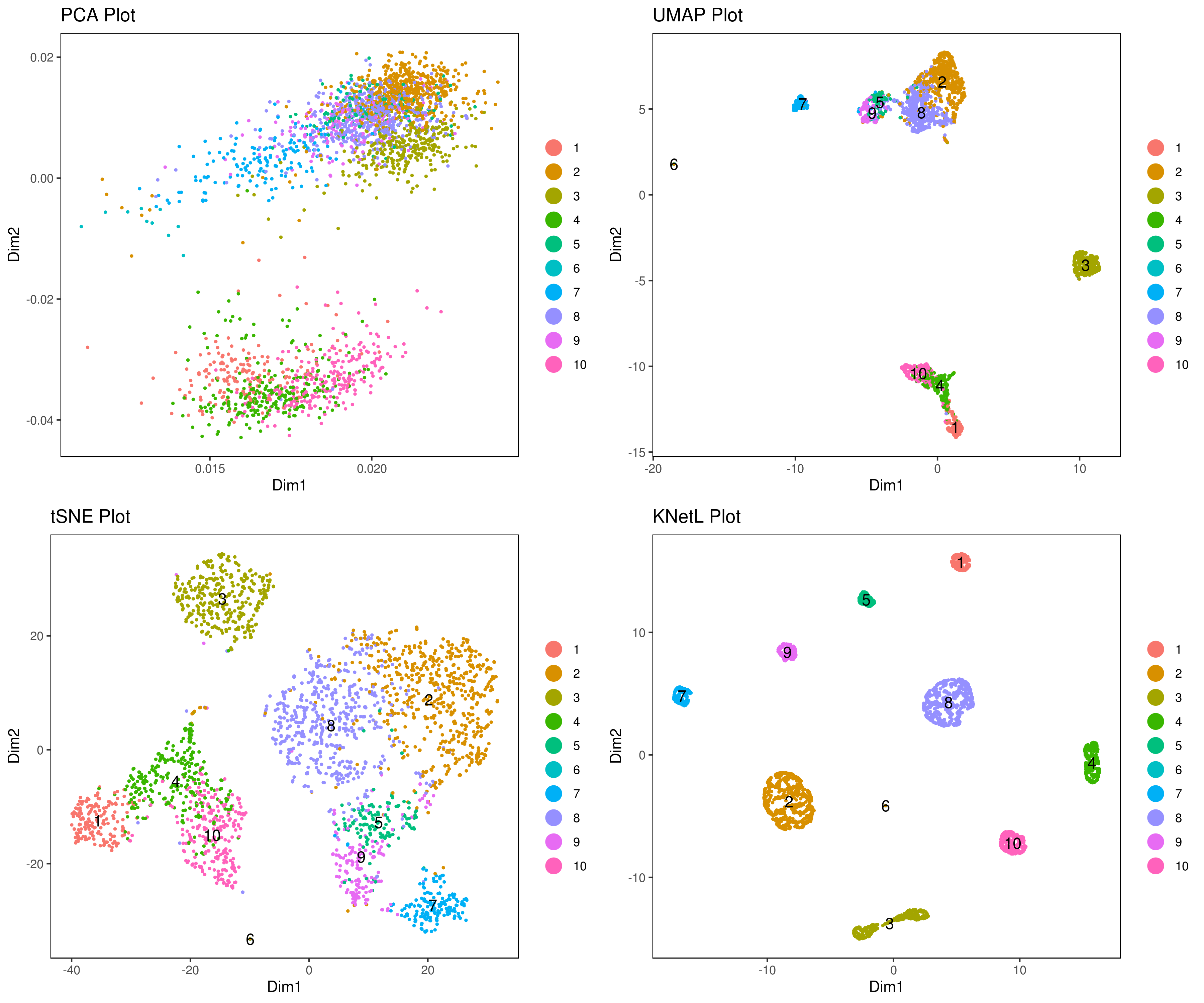
Visualize data clustering results

plot clusters (in the figures below clustering is done based on KNetL)

example: # my.obj <- iclust(my.obj, k = 150, data.type = "knetl")

A <- cluster.plot(my.obj,plot.type = "pca",interactive = F,cell.size = 0.5,cell.transparency = 1, anno.clust=T) B <- cluster.plot(my.obj,plot.type = "umap",interactive = F,cell.size = 0.5,cell.transparency = 1,anno.clust=T) C <- cluster.plot(my.obj,plot.type = "tsne",interactive = F,cell.size = 0.5,cell.transparency = 1,anno.clust=T) D <- cluster.plot(my.obj,plot.type = "knetl",interactive = F,cell.size = 0.5,cell.transparency = 1,anno.clust=T)

library(gridExtra) grid.arrange(A,B,C,D)

Re-numbering clusters based on their distances, this is so that the are more in consecutive order (optional)

This is visually helpful to look at your heatmap after finding marker genes and can help you decide which clusters need to be merged and adjusted.

my.obj <- clust.ord(my.obj,top.rank = 500, how.to.order = "distance") #my.obj <- clust.ord(my.obj,top.rank = 500, how.to.order = "random")

A= cluster.plot(my.obj,plot.type = "pca",interactive = F,cell.size = 0.5,cell.transparency = 1, anno.clust=T) B= cluster.plot(my.obj,plot.type = "umap",interactive = F,cell.size = 0.5,cell.transparency = 1,anno.clust=T) C= cluster.plot(my.obj,plot.type = "tsne",interactive = F,cell.size = 0.5,cell.transparency = 1,anno.clust=T) D= cluster.plot(my.obj,plot.type = "knetl",interactive = F,cell.size = 0.5,cell.transparency = 1,anno.clust=T)

library(gridExtra) grid.arrange(A,B,C,D)

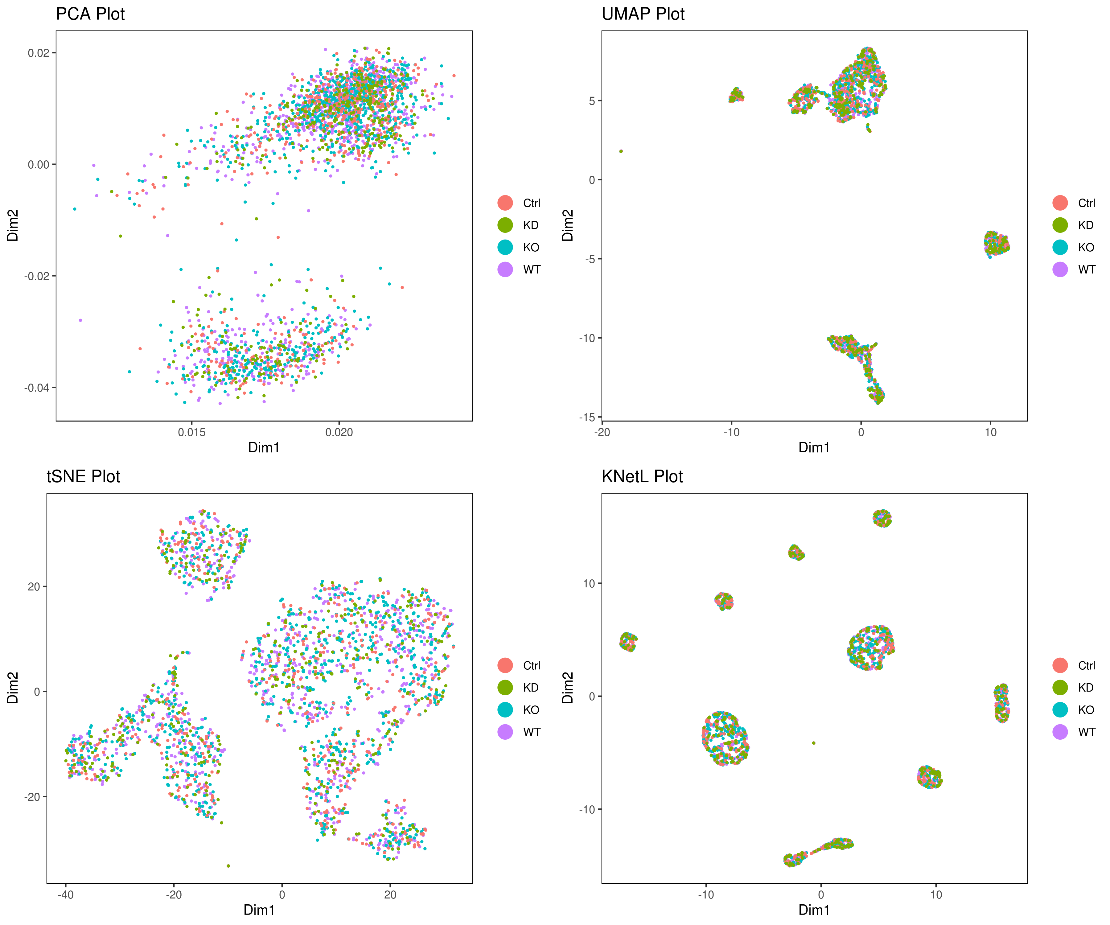
Look at conditions

conditions

A <- cluster.plot(my.obj,plot.type = "pca",col.by = "conditions",interactive = F,cell.size = 0.5) B <- cluster.plot(my.obj,plot.type = "umap",col.by = "conditions",interactive = F,cell.size = 0.5) C <- cluster.plot(my.obj,plot.type = "tsne",col.by = "conditions",interactive = F,cell.size = 0.5) D <- cluster.plot(my.obj,plot.type = "knetl",col.by = "conditions",interactive = F,cell.size = 0.5)

library(gridExtra) grid.arrange(A,B,C,D)

or

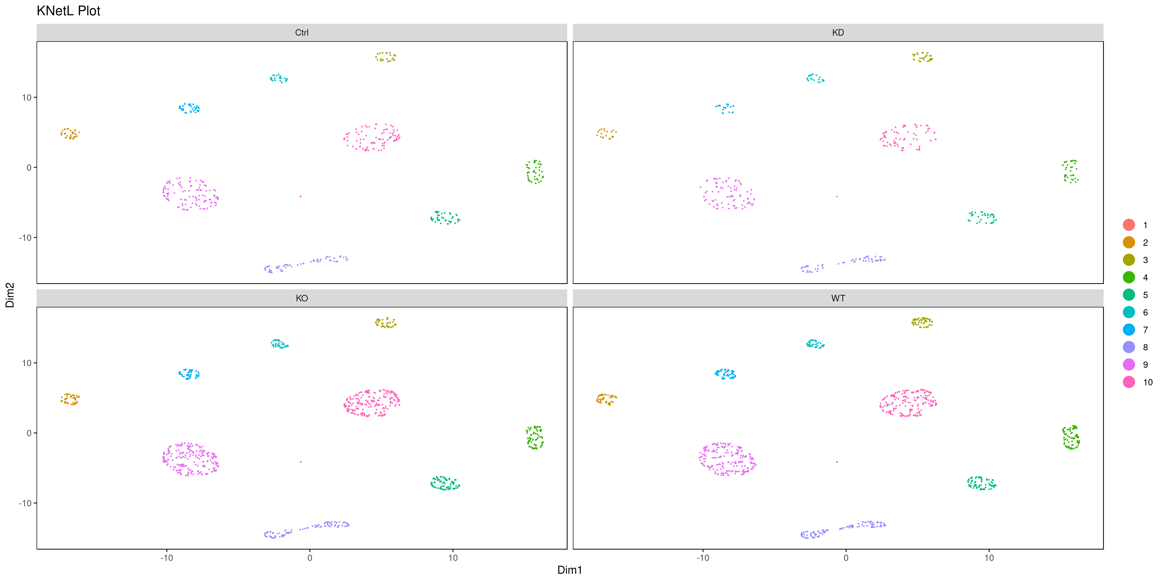
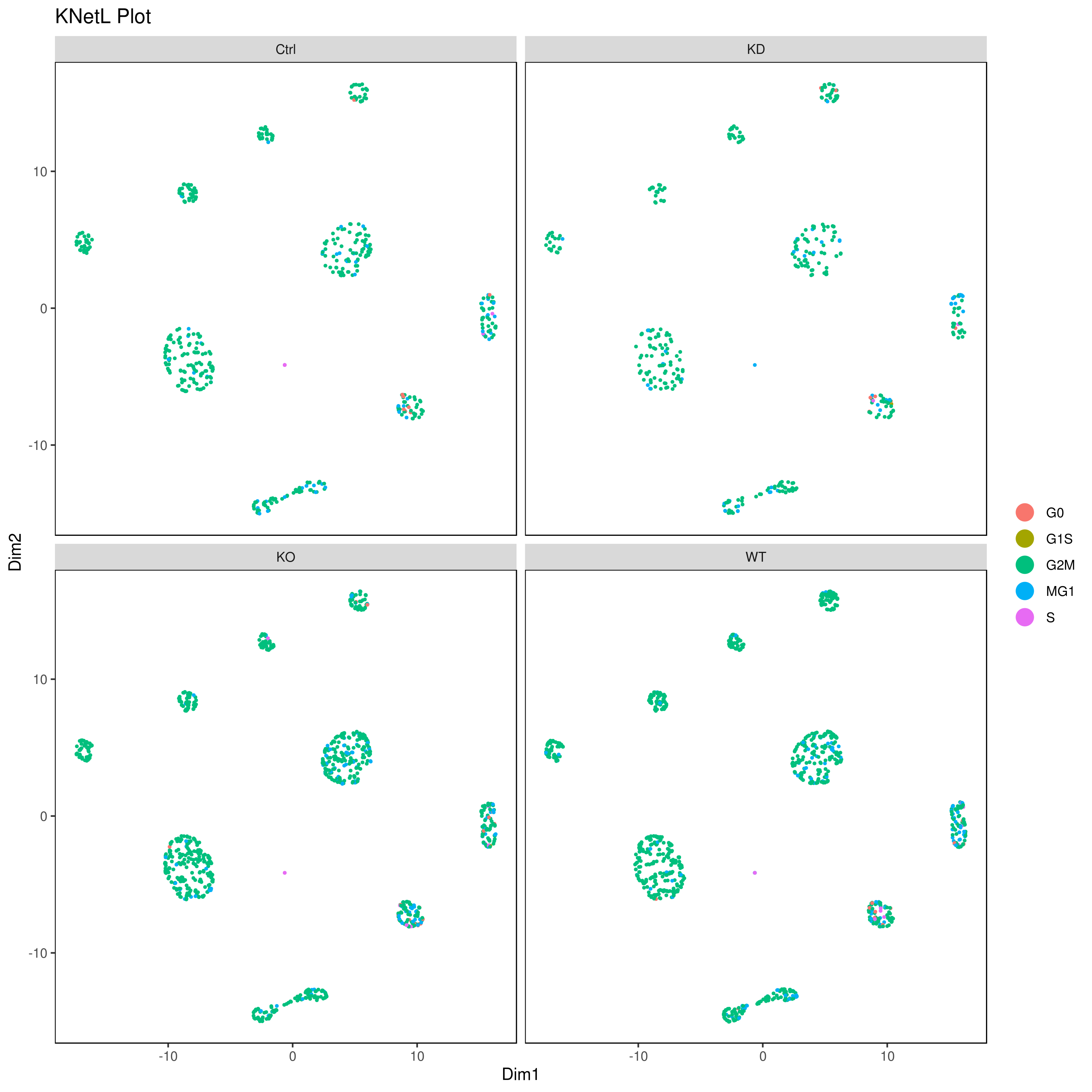
png('AllConds_clusts_knetl.png', width = 16, height = 8, units = 'in', res = 300) cluster.plot(my.obj, cell.size = 0.1, plot.type = "knetl", cell.color = "black", back.col = "white", cell.transparency = 1, clust.dim = 2, interactive = F,cond.facet = T) dev.off()

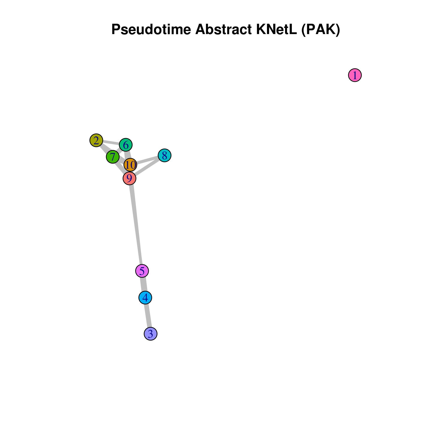
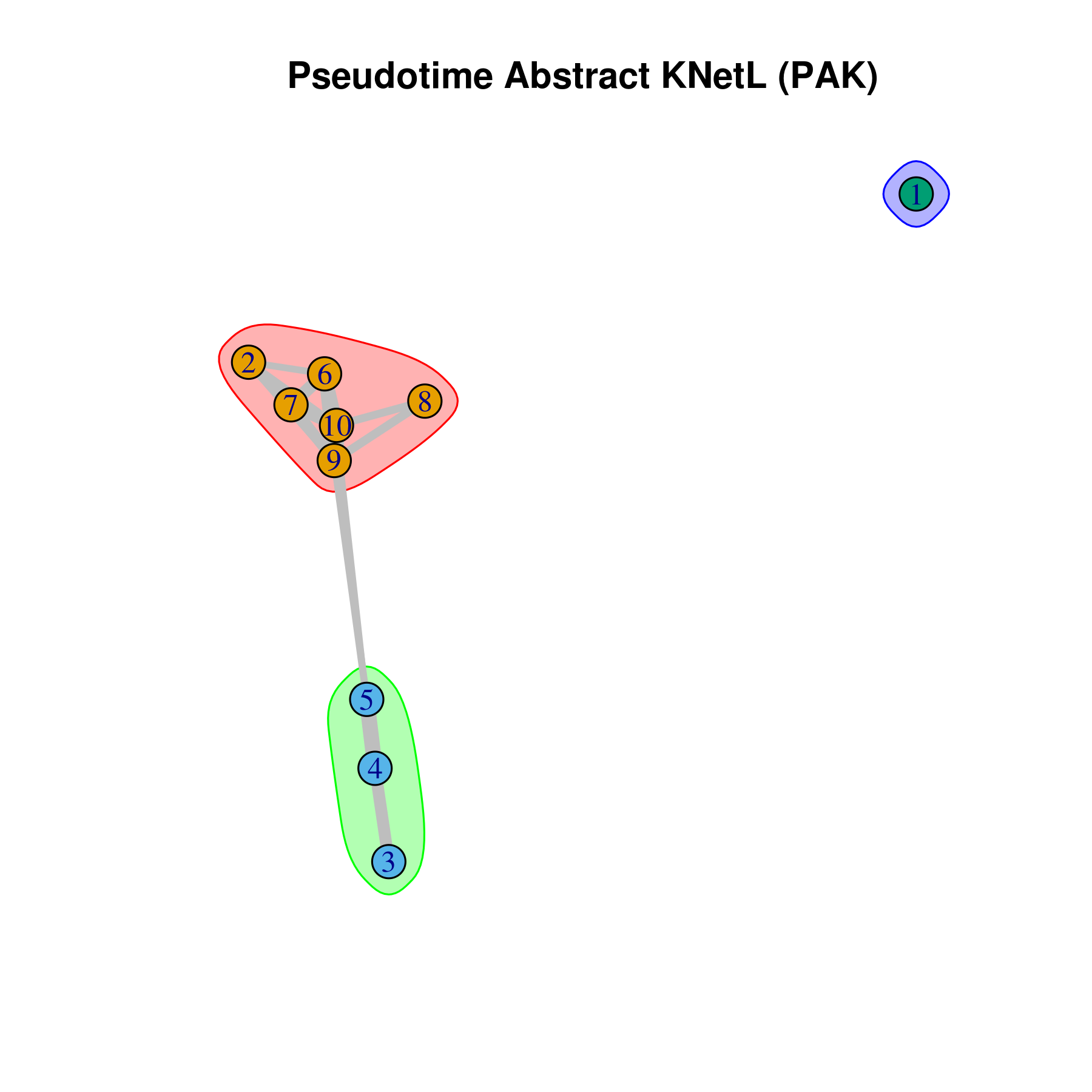
Pseudotime Abstract KNetL map (PAK map)

This is very helpful to see the distances or similarities between different communities. The shorter and thicker the lines/links (rubber bands) are the more similar the communities. The nodes are the clusters and the edges or links are the distance between them.

pseudotime.knetl(my.obj,interactive = F,cluster.membership = F,conds.to.plot = NULL)

with memberships

pseudotime.knetl(my.obj,interactive = F,cluster.membership = T,conds.to.plot = NULL)

intractive plot

pseudotime.knetl(my.obj,interactive = T)

Average expression per cluster

for all cunditions

my.obj <- clust.avg.exp(my.obj, conds.to.avg = NULL)

for one cundition

#my.obj <- clust.avg.exp(my.obj, conds.to.avg = "WT")

for two cundition

#my.obj <- clust.avg.exp(my.obj, conds.to.avg = c("WT","KO"))

head(my.obj@clust.avg)

gene cluster_1 cluster_2 cluster_3 cluster_4 cluster_5

#1 A1BG 0 0.034248447 0.029590643 0.076486590 0.090270833 #2 A1BG.AS1 0 0.000000000 0.006274854 0.019724138 0.004700000 #3 A1CF 0 0.000000000 0.000000000 0.000000000 0.000000000 #4 A2M 0 0.006925466 0.003614035 0.000000000 0.000000000 #5 A2M.AS1 0 0.056155280 0.000000000 0.005344828 0.006795833 #6 A2ML1 0 0.000000000 0.000000000 0.000000000 0.000000000

cluster_6 cluster_7 cluster_8 cluster_9 cluster_10

#1 0.074360294 0.07623494 0.04522321 0.088735057 0.065292818 #2 0.000000000 0.00000000 0.01553869 0.013072698 0.013550645 #3 0.000000000 0.00000000 0.00000000 0.000000000 0.000000000 #4 0.000000000 0.00000000 0.00000000 0.001810985 0.003200737 #5 0.008191176 0.06227108 0.00000000 0.011621971 0.012837937 #6 0.000000000 0.00000000 0.00000000 0.000000000 0.000000000

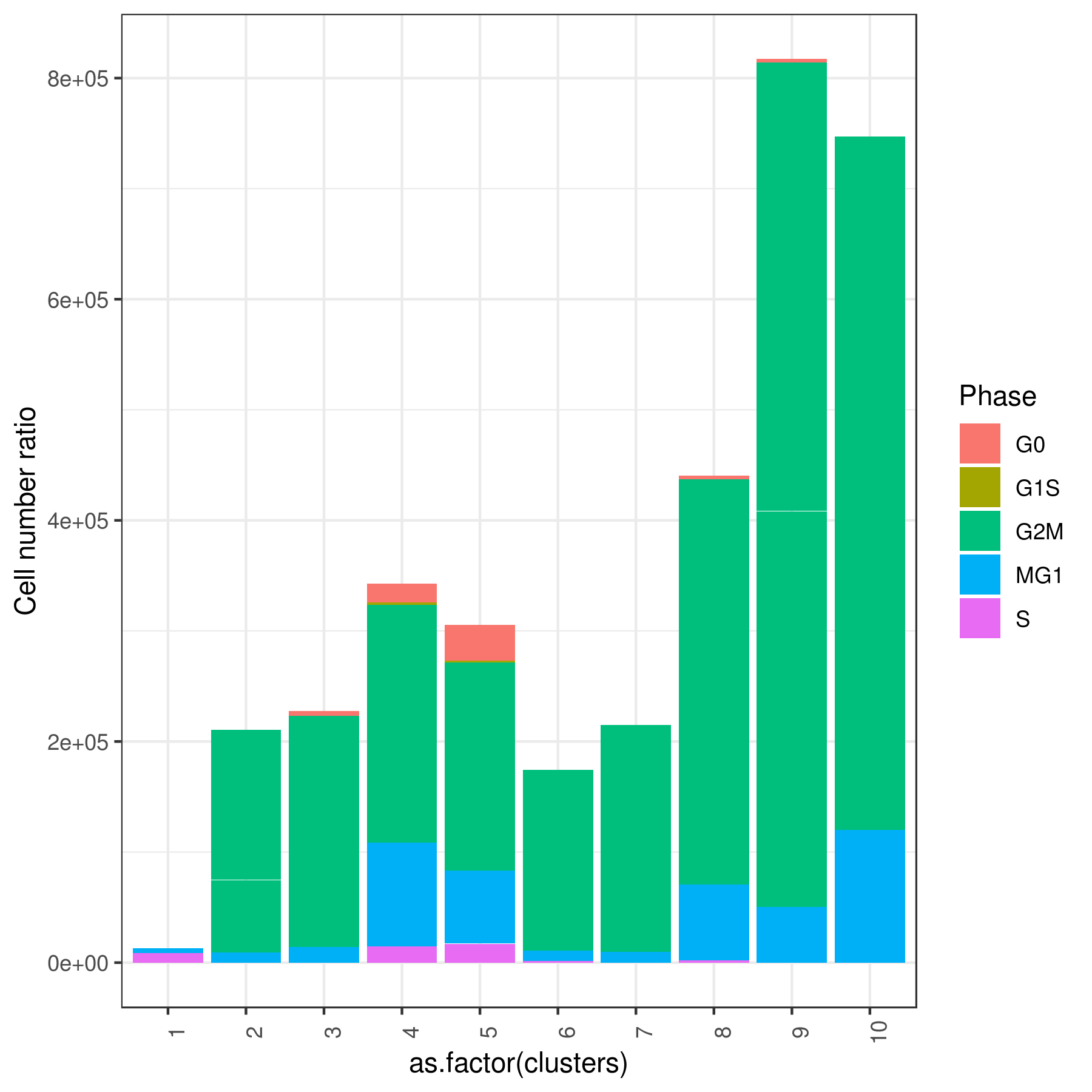
Cell cycle prediction

Tirosh scoring method Tirosh, et. al. 2016 (default) or coverage is used to calculate G0, G1S, G2M, M, G1M and S phase score. The gene lists for G0, G1S, G2M, M, G1M and S phase are chosen from previously published article Xue, et.al 2020

NOTE: These genes work best for cancer cells. You can use a different gene set for each category (G0, G1S, G2M, M, G1M and S).

old method

my.obj <- cc(my.obj, s.genes = s.phase, g2m.genes = g2m.phase)

new method

G0 <- readLines(system.file('extdata', 'G0.txt', package = 'iCellR')) G1S <- readLines(system.file('extdata', 'G1S.txt', package = 'iCellR')) G2M <- readLines(system.file('extdata', 'G2M.txt', package = 'iCellR')) M <- readLines(system.file('extdata', 'M.txt', package = 'iCellR')) MG1 <- readLines(system.file('extdata', 'MG1.txt', package = 'iCellR')) S <- readLines(system.file('extdata', 'S.txt', package = 'iCellR'))

Tirosh scoring method (recomanded)

my.obj <- cell.cycle(my.obj, scoring.List = c("G0","G1S","G2M","M","MG1","S"), scoring.method = "tirosh")

Coverage scoring method (recomanded)

my.obj <- cell.cycle(my.obj, scoring.List = c("G0","G1S","G2M","M","MG1","S"), scoring.method = "coverage")

plot cell cycle

A= cluster.plot(my.obj,plot.type = "pca",interactive = F,cell.size = 0.5,cell.transparency = 1, anno.clust=T,col.by = "cc") B= cluster.plot(my.obj,plot.type = "umap",interactive = F,cell.size = 0.5,cell.transparency = 1,anno.clust=T, col.by = "cc") C= cluster.plot(my.obj,plot.type = "tsne",interactive = F,cell.size = 0.5,cell.transparency = 1,anno.clust=T, col.by = "cc") D= cluster.plot(my.obj,plot.type = "knetl",interactive = F,cell.size = 0.5,cell.transparency = 1,anno.clust=T, col.by = "cc")

library(gridExtra) grid.arrange(A,B,C,D)

or

cluster.plot(my.obj, cell.size = 0.5, plot.type = "knetl", col.by = "cc", cell.color = "black", back.col = "white", cell.transparency = 1, clust.dim = 2, interactive = F,cond.facet = T)

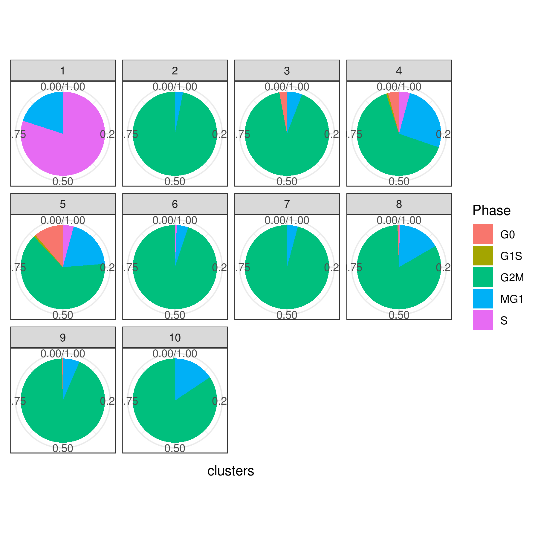
Pie

clust.stats.plot(my.obj, plot.type = "pie.cc", interactive = F, conds.to.plot = NULL) dev.off()

bar

clust.stats.plot(my.obj, plot.type = "bar.cc", interactive = F, conds.to.plot = NULL) dev.off()

or per condition

clust.stats.plot(my.obj, plot.type = "pie.cc", interactive = F, conds.to.plot = "WT")

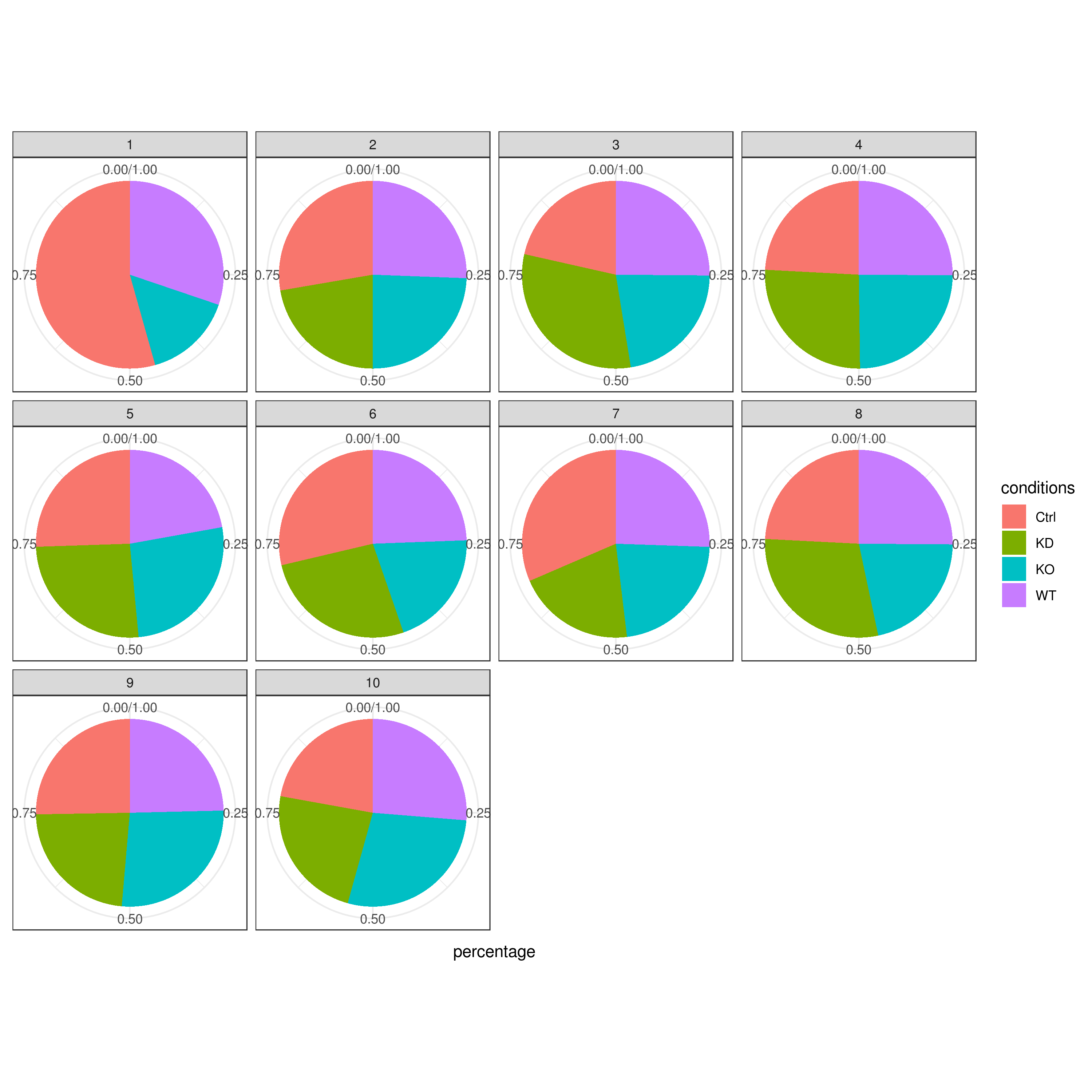
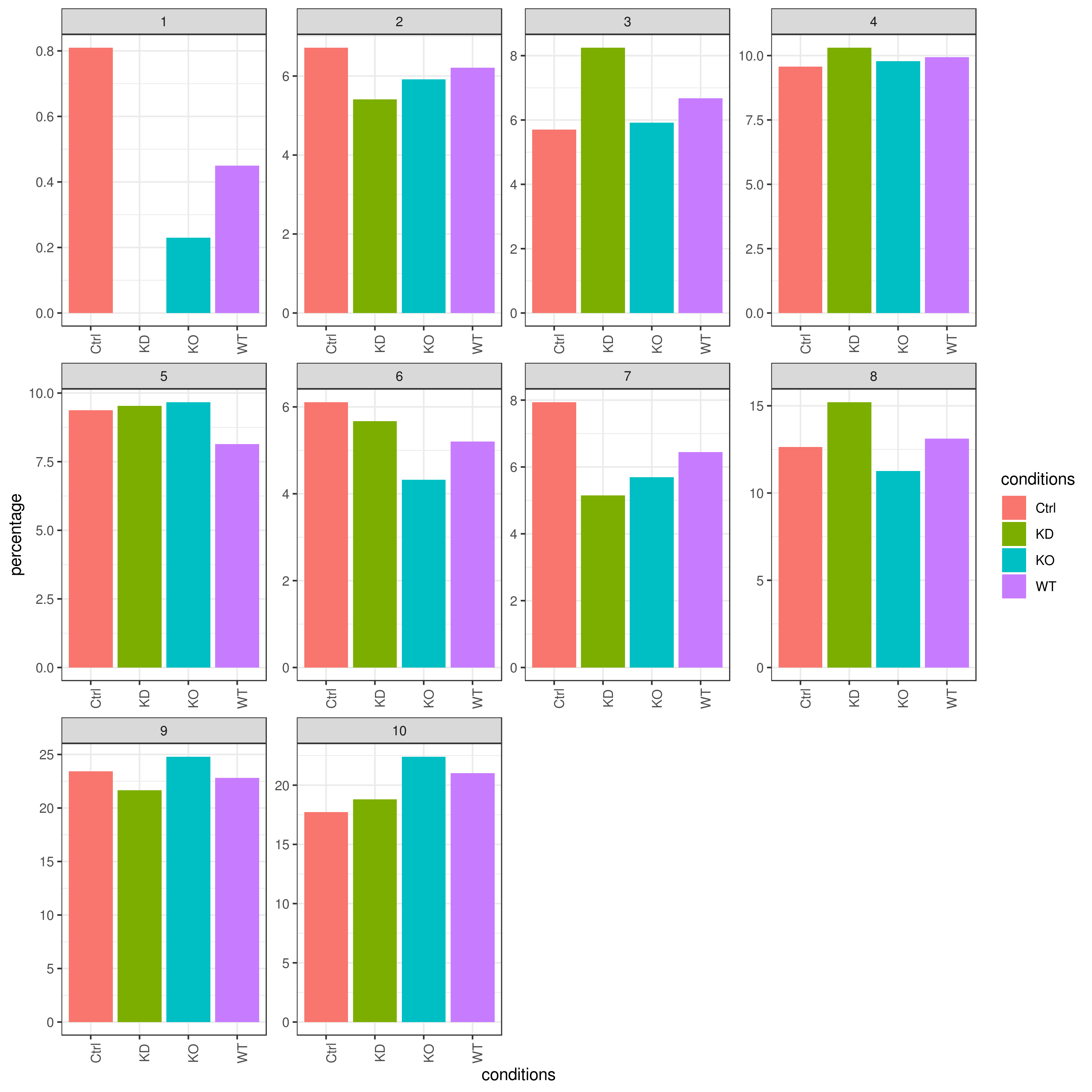
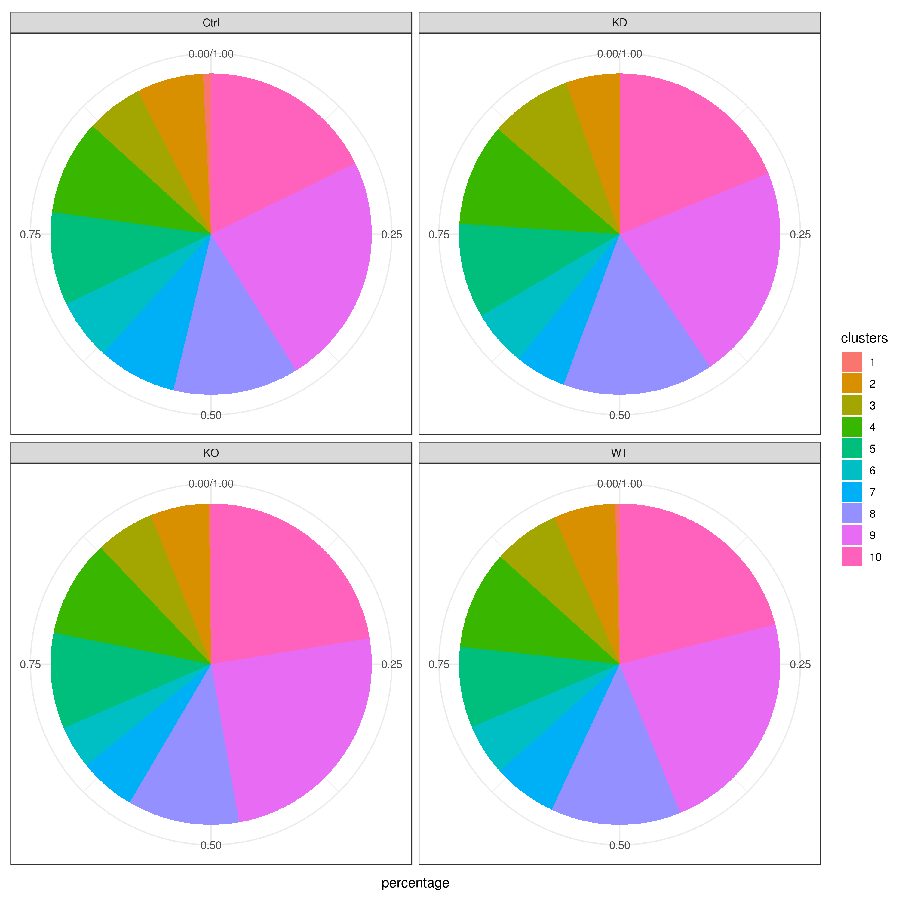
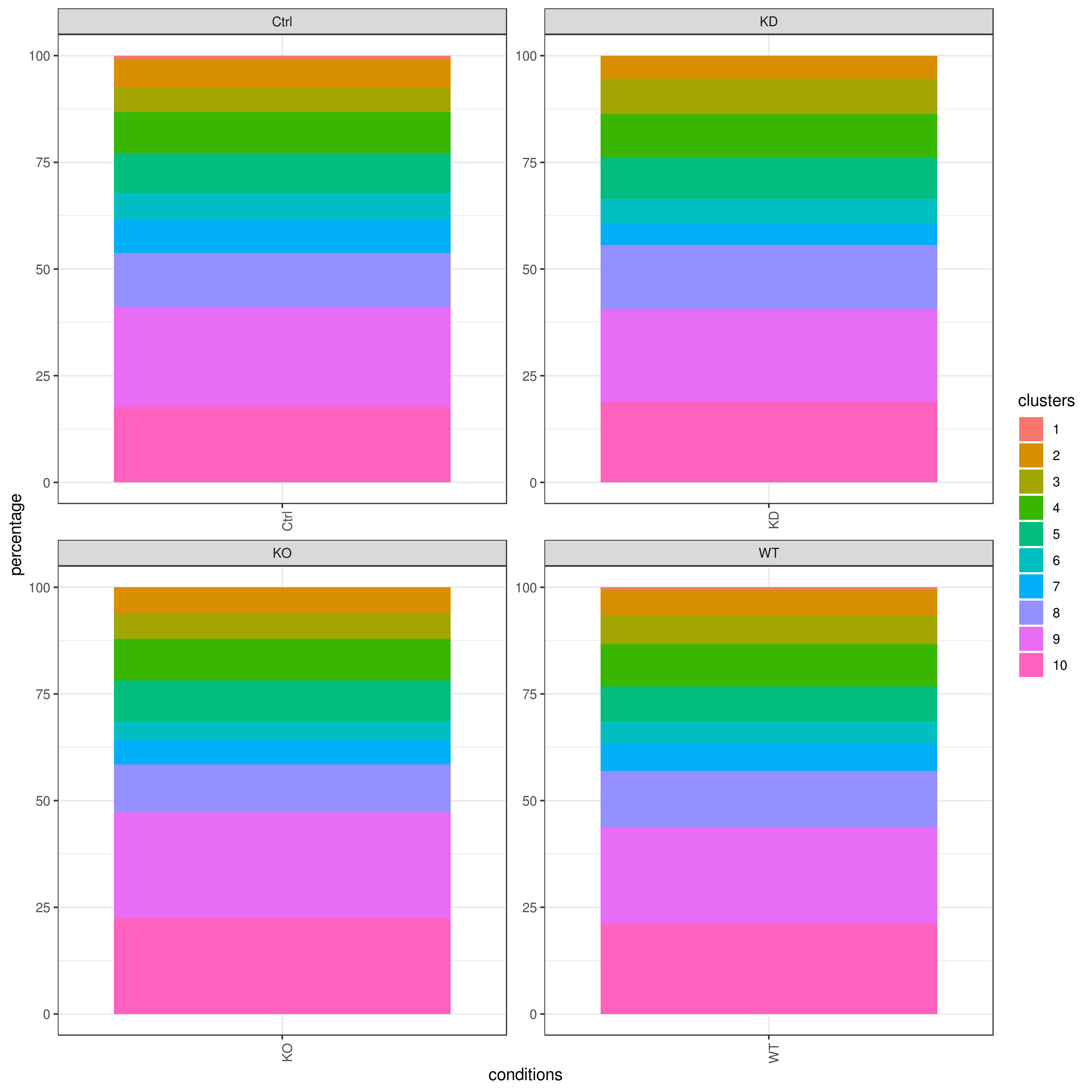
Cell frequencies and proportions

clust.cond.info(my.obj, plot.type = "pie", normalize.ncell = TRUE, my.out.put = "plot", normalize.by = "percentage")

clust.cond.info(my.obj, plot.type = "bar", normalize.ncell = TRUE,my.out.put = "plot", normalize.by = "percentage")

clust.cond.info(my.obj, plot.type = "pie.cond", normalize.ncell = T, my.out.put = "plot", normalize.by = "percentage")

clust.cond.info(my.obj, plot.type = "bar.cond", normalize.ncell = T,my.out.put = "plot", normalize.by = "percentage")

my.obj <- clust.cond.info(my.obj) head(my.obj@my.freq)

conditions TC SF clusters Freq Norm.Freq percentage

#1 Ctrl 491 1.265 1 4 3.162 0.81 #2 Ctrl 491 1.265 11 32 25.296 6.52 #3 Ctrl 491 1.265 8 114 90.119 23.22 #4 Ctrl 491 1.265 5 43 33.992 8.76 #5 Ctrl 491 1.265 2 33 26.087 6.72 #6 Ctrl 491 1.265 9 86 67.984 17.52

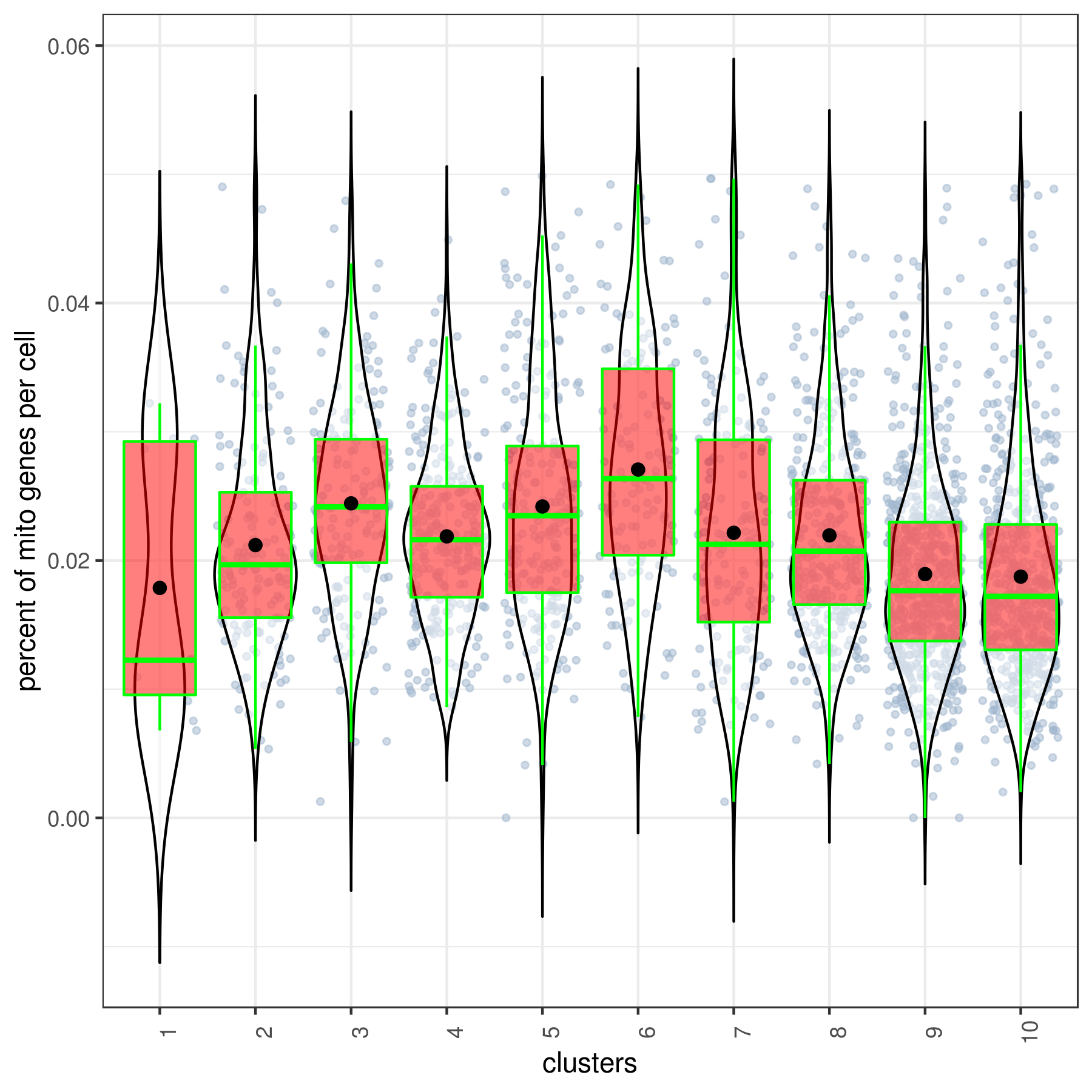
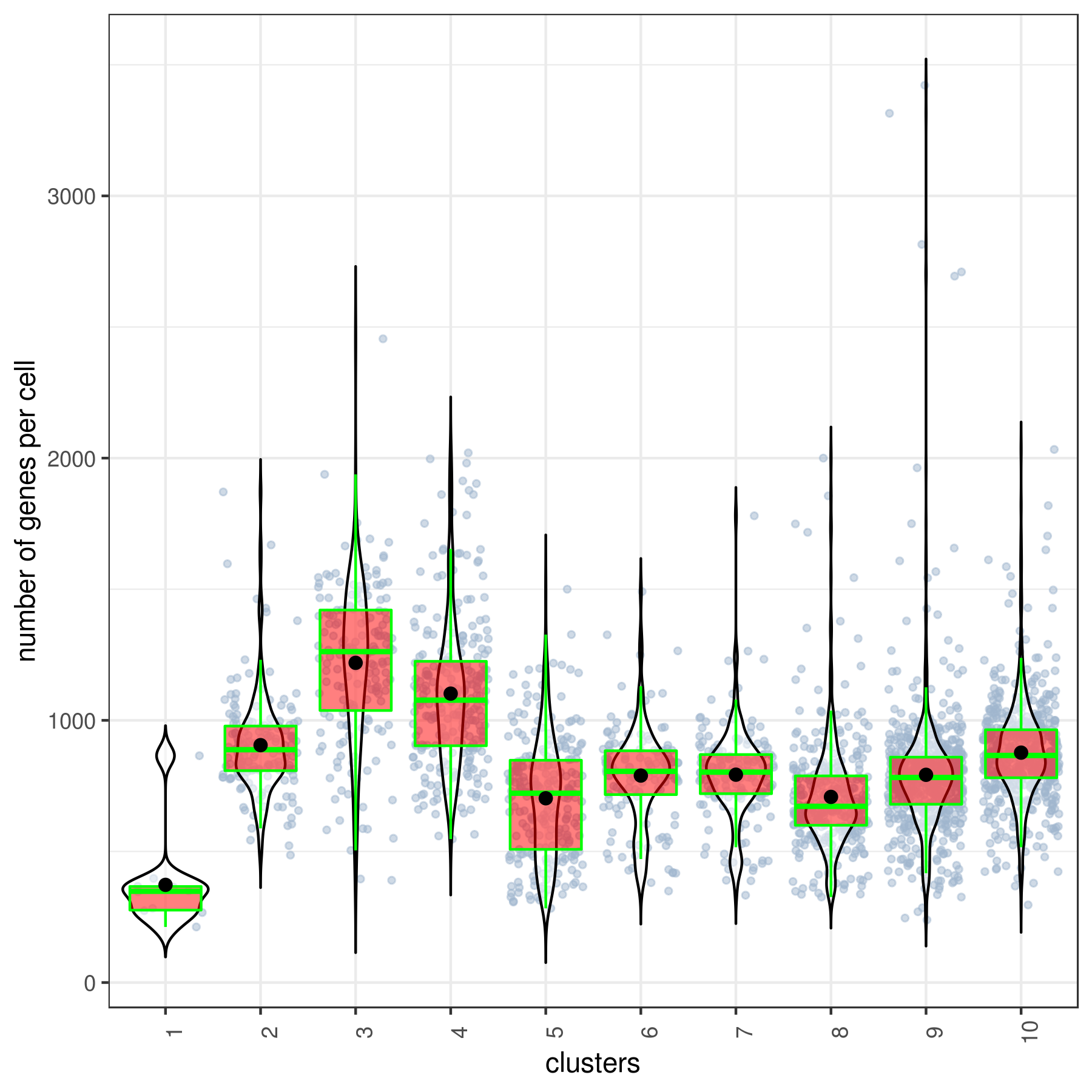
Cluster QC

clust.stats.plot(my.obj, plot.type = "box.mito", interactive = F)

clust.stats.plot(my.obj, plot.type = "box.gene", interactive = F)

Run data imputation

my.obj <- run.impute(my.obj, dims = 1:10, nn = 10, data.type = "pca")

Save your object

save(my.obj, file = "my.obj.Robj")

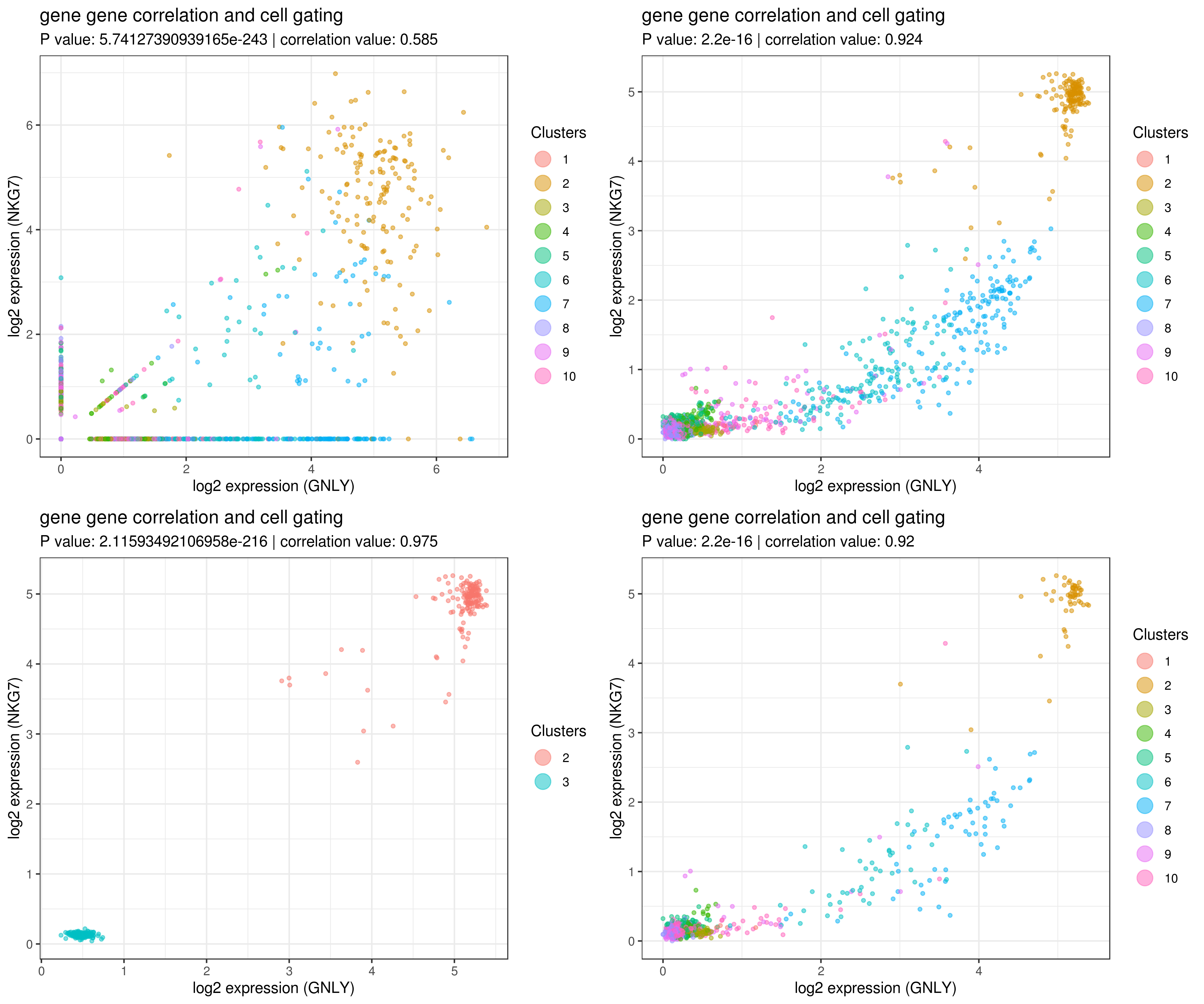
gene gene correlation

impute more cells by increasing nn for better resulst.

my.obj <- run.impute(my.obj,dims = 1:10,data.type = "pca", nn = 50)

main data

A <- gg.cor(my.obj, interactive = F, gene1 = "GNLY", gene2 = "NKG7", conds = NULL, clusts = NULL, data.type = "main")

imputed data

B <- gg.cor(my.obj, interactive = F, gene1 = "GNLY", gene2 = "NKG7", conds = NULL, clusts = NULL, data.type = "imputed")

C <- gg.cor(my.obj, interactive = F, gene1 = "GNLY", gene2 = "NKG7", conds = NULL, clusts = c(3,2), data.type = "imputed")

imputed data

D <- gg.cor(my.obj, interactive = F, gene1 = "GNLY", gene2 = "NKG7", conds = c("WT"), clusts = NULL, data.type = "imputed")

grid.arrange(A,B,C,D)

Find marker genes

marker.genes <- findMarkers(my.obj, fold.change = 2, padjval = 0.1)

dim(marker.genes)

[1] 1070 17

head(marker.genes)

baseMean baseSD AvExpInCluster AvExpInOtherClusters foldChange

#PPBP 0.8257760 12.144694 181.3945 0.1399852 1295.8120969 #GPX1 1.3989591 4.344717 57.4034 1.1862571 48.3903523 #CALM3 0.5469743 1.230942 10.7848 0.5080915 21.2260968 #OAZ1 4.9077851 5.979586 46.7867 4.7487311 9.8524635 #MYL6 3.0806167 3.562124 21.3690 3.0111584 7.0966045 #CD74 8.5523704 13.359205 2.6120 8.5749316 0.3046088

log2FoldChange pval padj clusters gene cluster_1

#PPBP 10.339641 1.586683e-06 0.014786300 1 PPBP 181.3945 #GPX1 5.596648 1.107541e-07 0.001103775 1 GPX1 57.4034 #CALM3 4.407767 2.098341e-06 0.019415953 1 CALM3 10.7848 #OAZ1 3.300485 7.857814e-07 0.007464137 1 OAZ1 46.7867 #MYL6 2.827129 1.296112e-06 0.012156230 1 MYL6 21.3690 #CD74 -1.714970 9.505749e-06 0.083983296 1 CD74 2.6120

cluster_2 cluster_3 cluster_4 cluster_5 cluster_6 cluster_7

#PPBP 0.0000000 0.1444327 0.2282912 0.0640625 0.01739706 0.1541084 #GPX1 0.2424969 1.2218772 3.9292720 4.4329583 0.25663235 0.2712831 #CALM3 0.6537205 0.8149415 0.6071034 0.5245625 0.44687500 0.5081867 #OAZ1 3.2077826 12.2072339 8.6080077 10.8738208 2.71288971 3.6402289 #MYL6 4.9660870 5.7945673 4.2813218 4.3046458 2.42854412 3.9030542 #CD74 2.9385839 8.9848538 15.7646245 5.9454250 2.19555882 3.8323072

cluster_8 cluster_9 cluster_10

#PPBP 0.02478274 0.3668433 0.01026335 #GPX1 0.61210714 0.4635153 0.39311786 #CALM3 0.22591369 0.5210339 0.48856538 #OAZ1 3.67225595 2.3590420 2.53362063 #MYL6 1.72344048 1.6460420 2.59901289 #CD74 36.10877976 1.5638853 1.82587477

baseMean: average expression in all the cells

baseSD: Standard Deviation

AvExpInCluster: average expression in cluster number (see clusters)

AvExpInOtherClusters: average expression in all the other clusters

foldChange: AvExpInCluster/AvExpInOtherClusters

log2FoldChange: log2(AvExpInCluster/AvExpInOtherClusters)

pval: P value

padj: Adjusted P value

clusters: marker for cluster number

gene: marker gene for the cluster

the rest are the average expression for each cluster

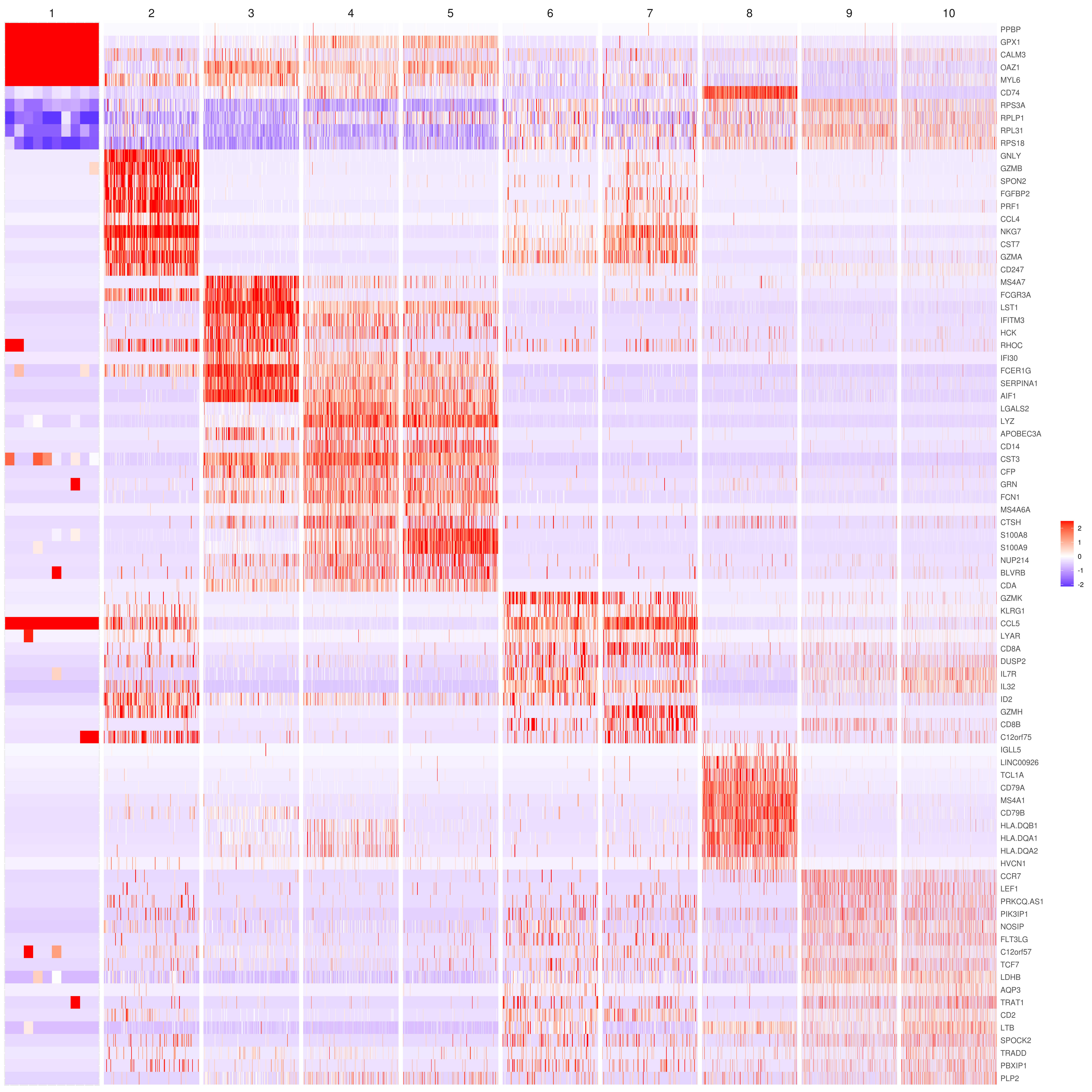
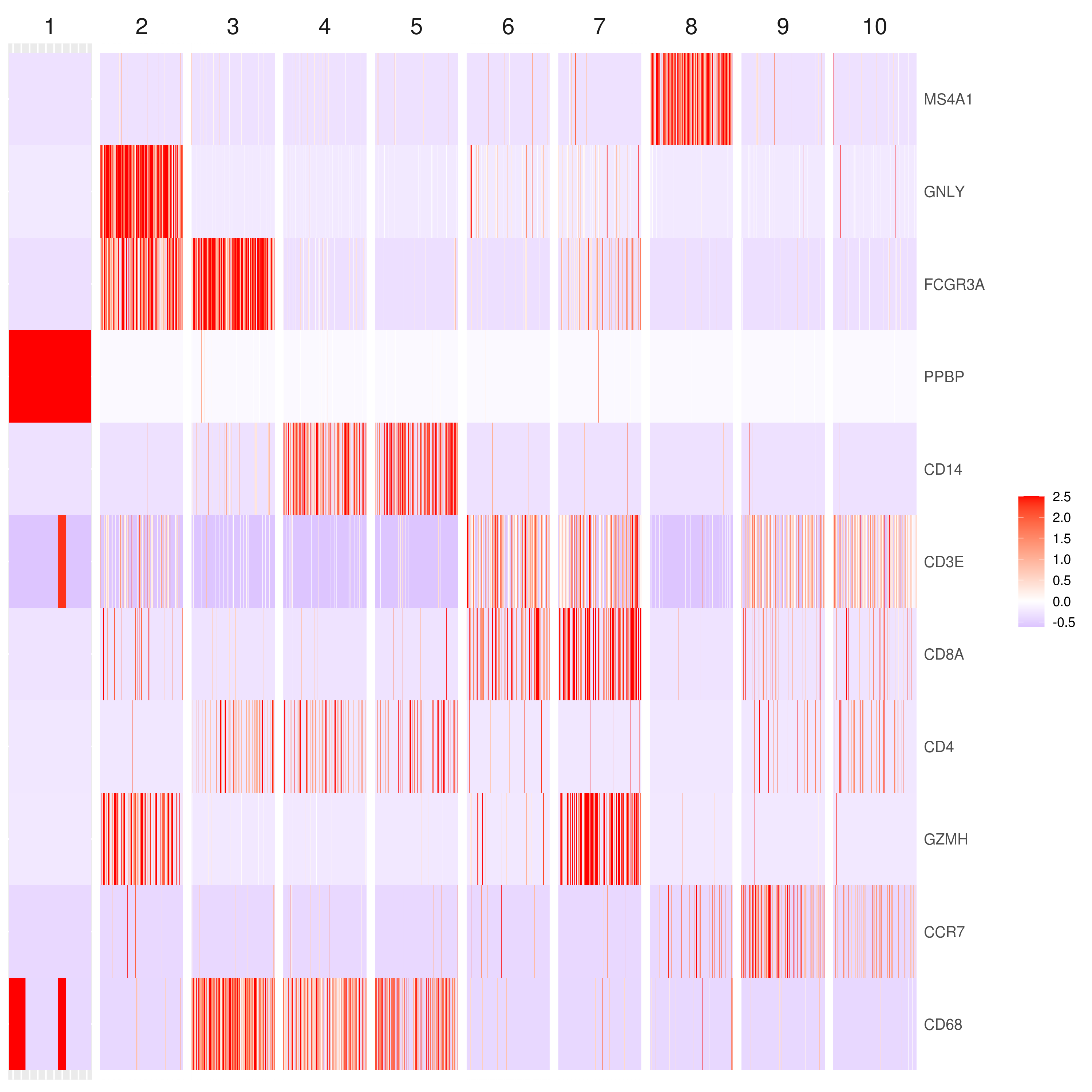
Heatmap

find top genes

MyGenes <- top.markers(marker.genes, topde = 10, min.base.mean = 0.2,filt.ambig = F) MyGenes <- unique(MyGenes)

main data

heatmap.gg.plot(my.obj, gene = MyGenes, interactive = F, cluster.by = "clusters", conds.to.plot = NULL)

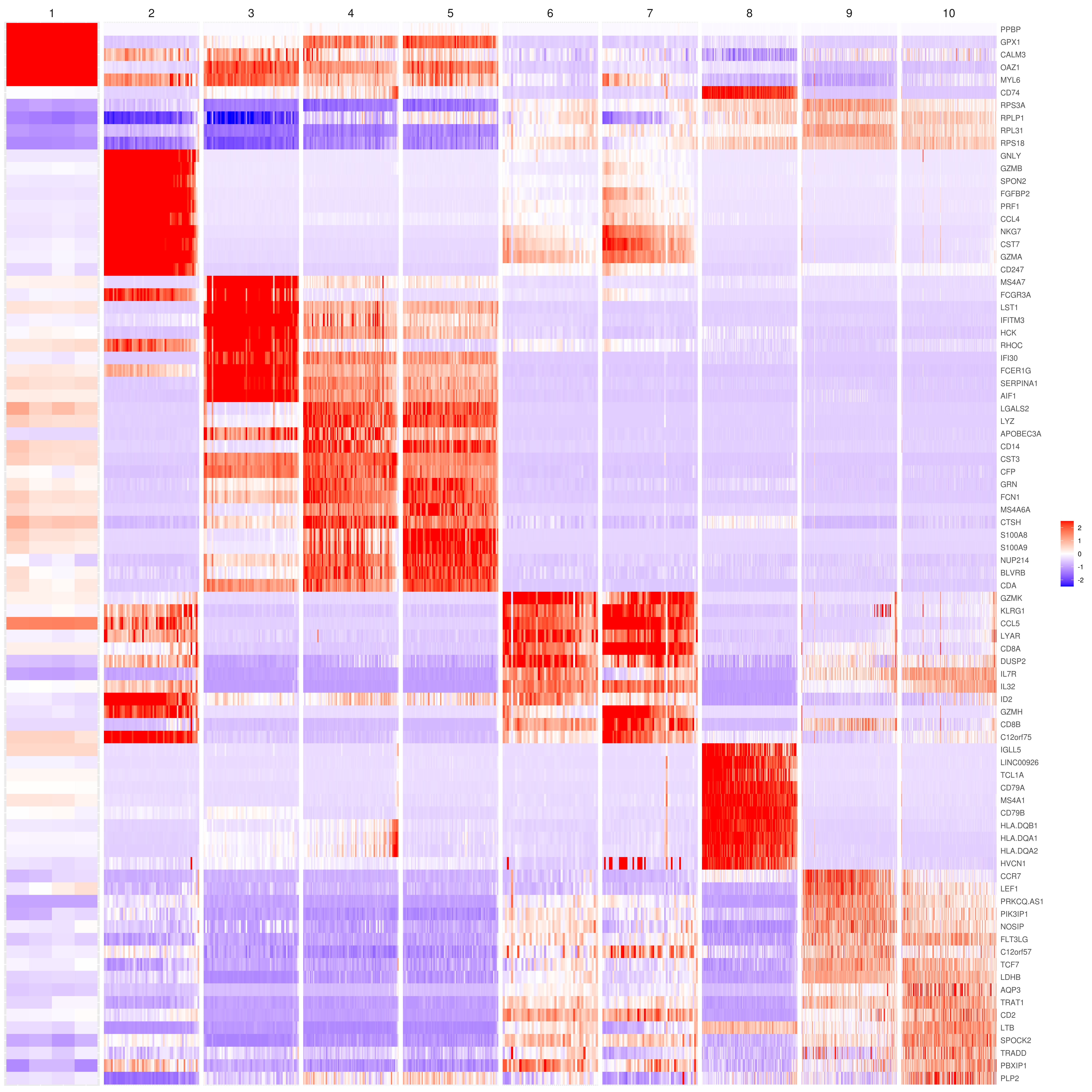
imputed data

heatmap.gg.plot(my.obj, gene = MyGenes, interactive = F, cluster.by = "clusters", data.type = "imputed", conds.to.plot = NULL)

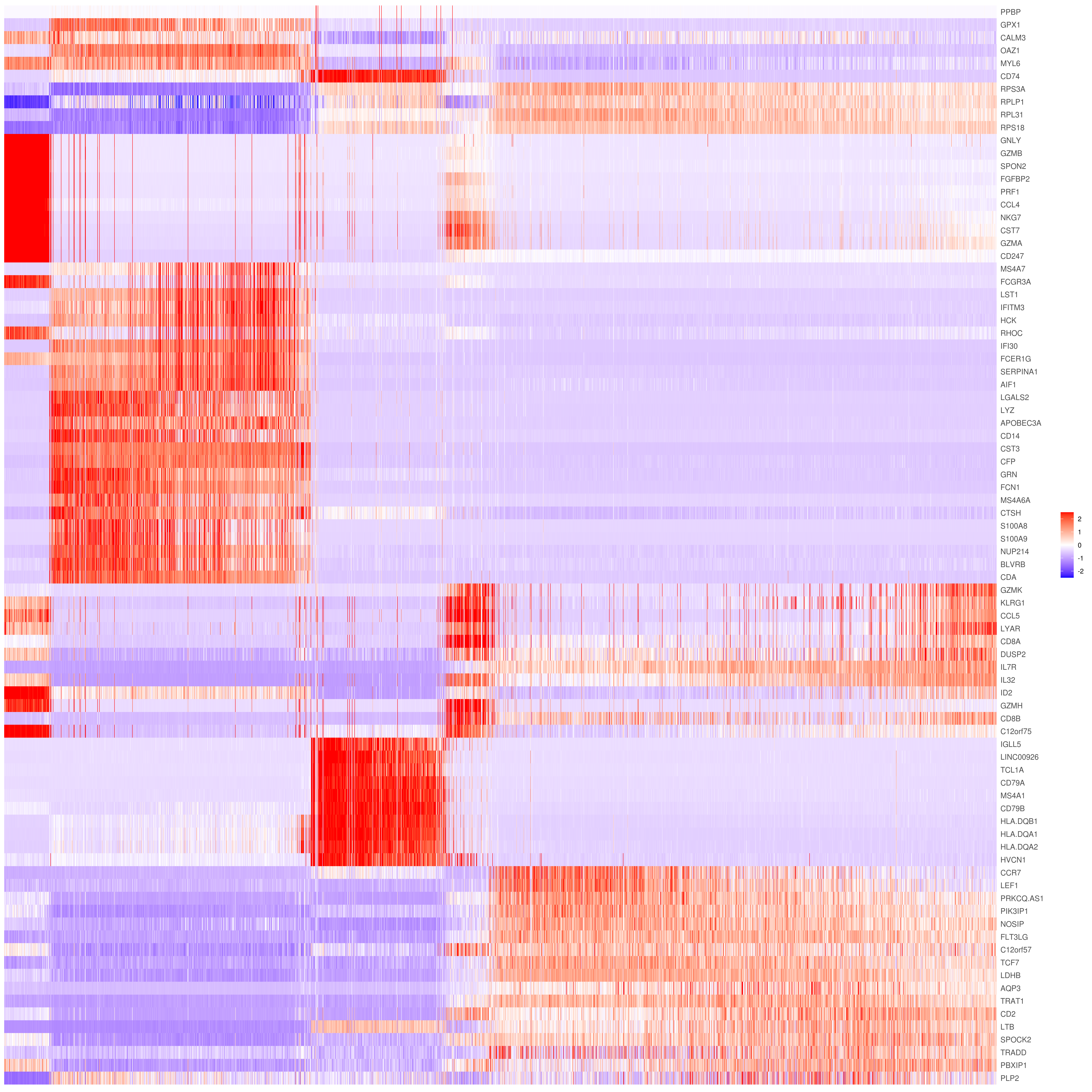
sort cells and plot only one condition

heatmap.gg.plot(my.obj, gene = MyGenes, interactive = F, cluster.by = "clusters", data.type = "imputed", cell.sort = TRUE, conds.to.plot = c("WT"))

Pseudotime stile

heatmap.gg.plot(my.obj, gene = MyGenes, interactive = F, cluster.by = "none", data.type = "imputed", cell.sort = TRUE)

intractive

heatmap.gg.plot(my.obj, gene = MyGenes, interactive = T, out.name = "heatmap_gg", cluster.by = "clusters")

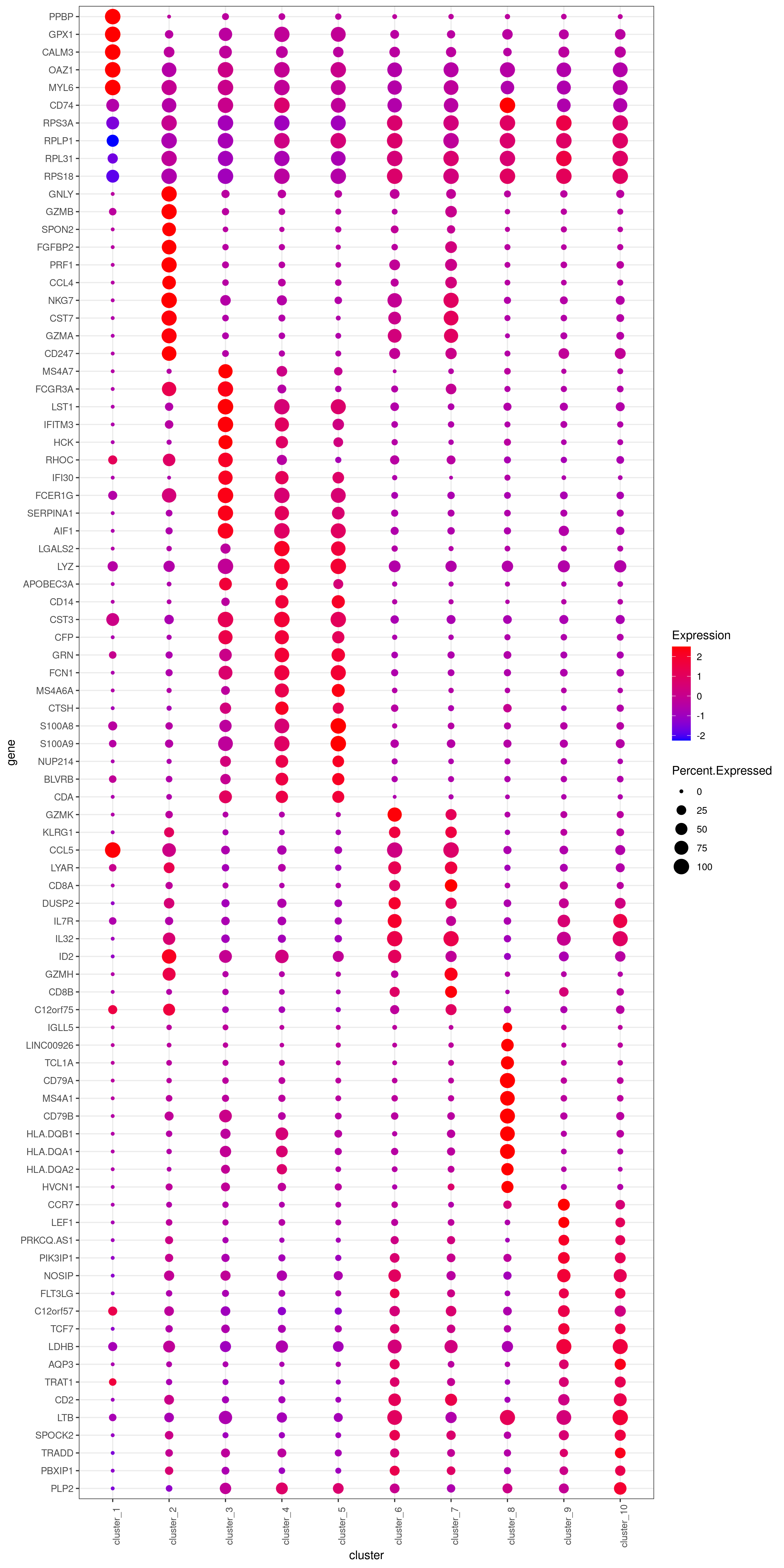
Bubble heatmap

png('heatmap_bubble_gg_genes.png', width = 10, height = 20, units = 'in', res = 300) bubble.gg.plot(my.obj, gene = MyGenes, interactive = F, conds.to.plot = NULL, size = "Percent.Expressed",colour = "Expression") dev.off()

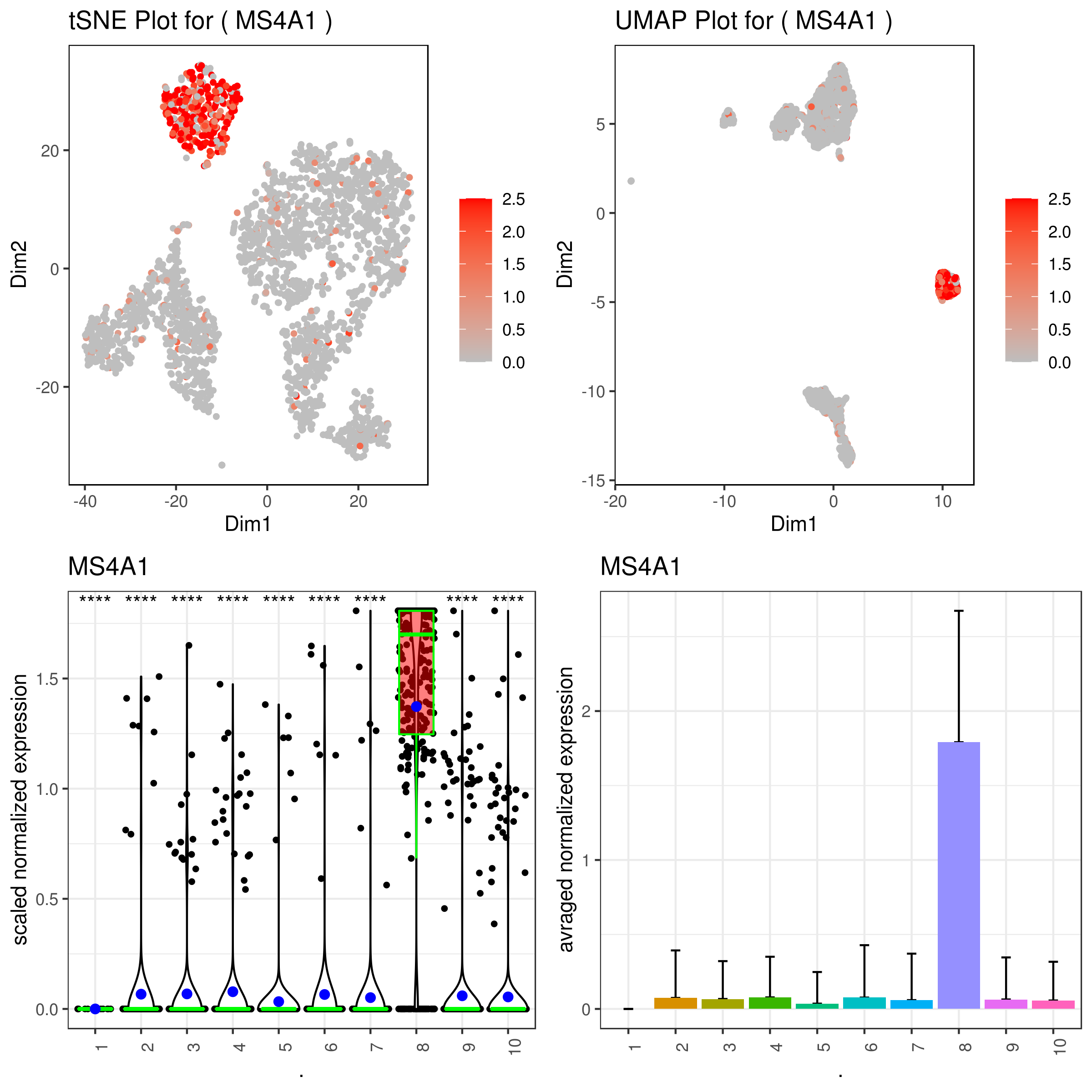
Plot genes

A <- gene.plot(my.obj, gene = "MS4A1", plot.type = "scatterplot", interactive = F, out.name = "scatter_plot")

PCA 2D

B <- gene.plot(my.obj, gene = "MS4A1", plot.type = "scatterplot", interactive = F, out.name = "scatter_plot", plot.data.type = "umap")

Box Plot

C <- gene.plot(my.obj, gene = "MS4A1", box.to.test = 0, box.pval = "sig.signs", col.by = "clusters", plot.type = "boxplot", interactive = F, out.name = "box_plot")

Bar plot (to visualize fold changes)

D <- gene.plot(my.obj, gene = "MS4A1", col.by = "clusters", plot.type = "barplot", interactive = F, out.name = "bar_plot")

library(gridExtra) png('gene.plots.png', width = 8, height = 8, units = 'in', res = 300) grid.arrange(A,B,C,D) dev.off()

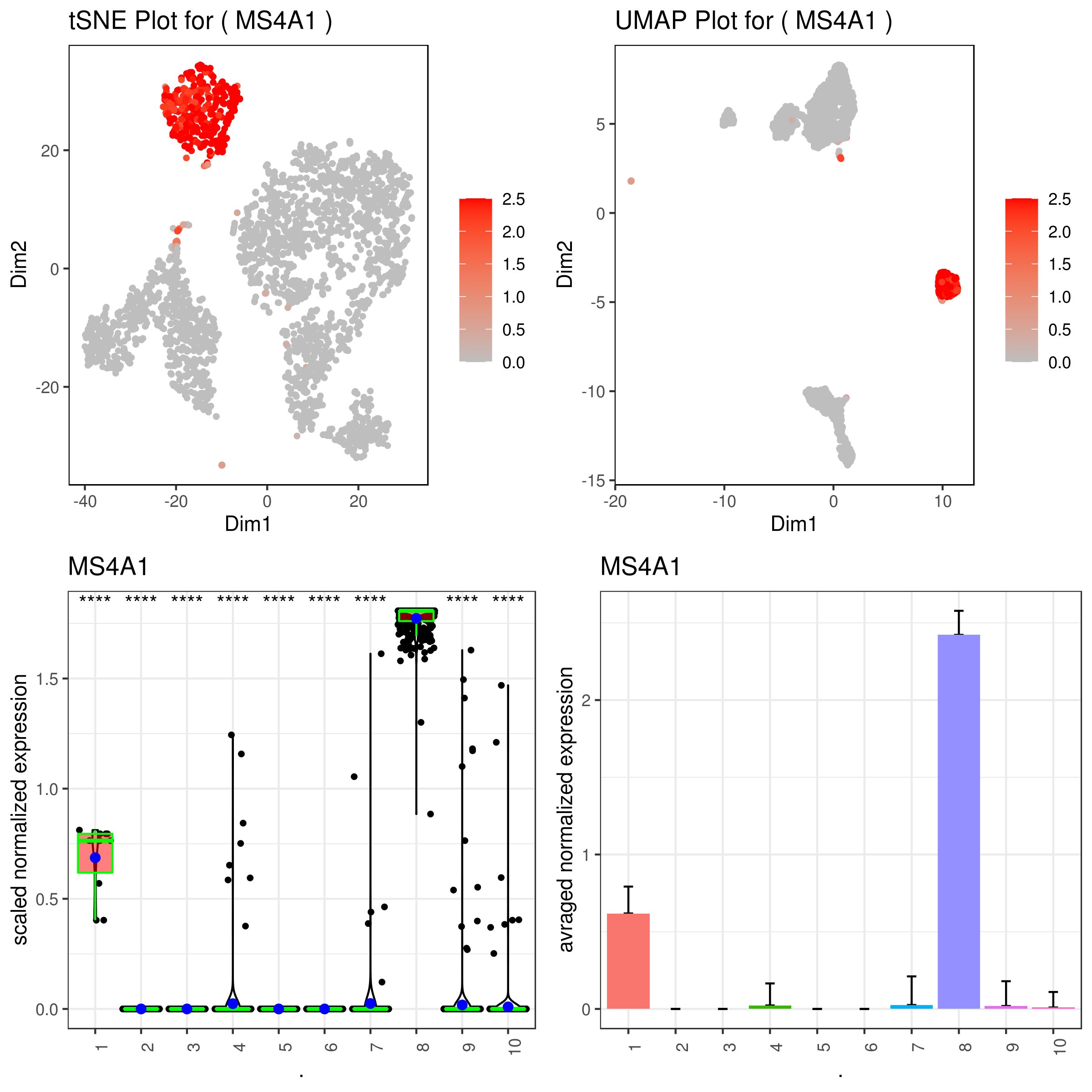
same on imputed data

A <- gene.plot(my.obj, gene = "MS4A1", plot.type = "scatterplot", interactive = F, data.type = "imputed", out.name = "scatter_plot")

PCA 2D

B <- gene.plot(my.obj, gene = "MS4A1", plot.type = "scatterplot", interactive = F, out.name = "scatter_plot", data.type = "imputed", plot.data.type = "umap")

Box Plot

C <- gene.plot(my.obj, gene = "MS4A1", box.to.test = 0, box.pval = "sig.signs", col.by = "clusters", plot.type = "boxplot", interactive = F, data.type = "imputed", out.name = "box_plot")

Bar plot (to visualize fold changes)

D <- gene.plot(my.obj, gene = "MS4A1", col.by = "clusters", plot.type = "barplot", interactive = F, data.type = "imputed", out.name = "bar_plot")

library(gridExtra) png('gene.plots_imputed.png', width = 8, height = 8, units = 'in', res = 300) grid.arrange(A,B,C,D) dev.off()

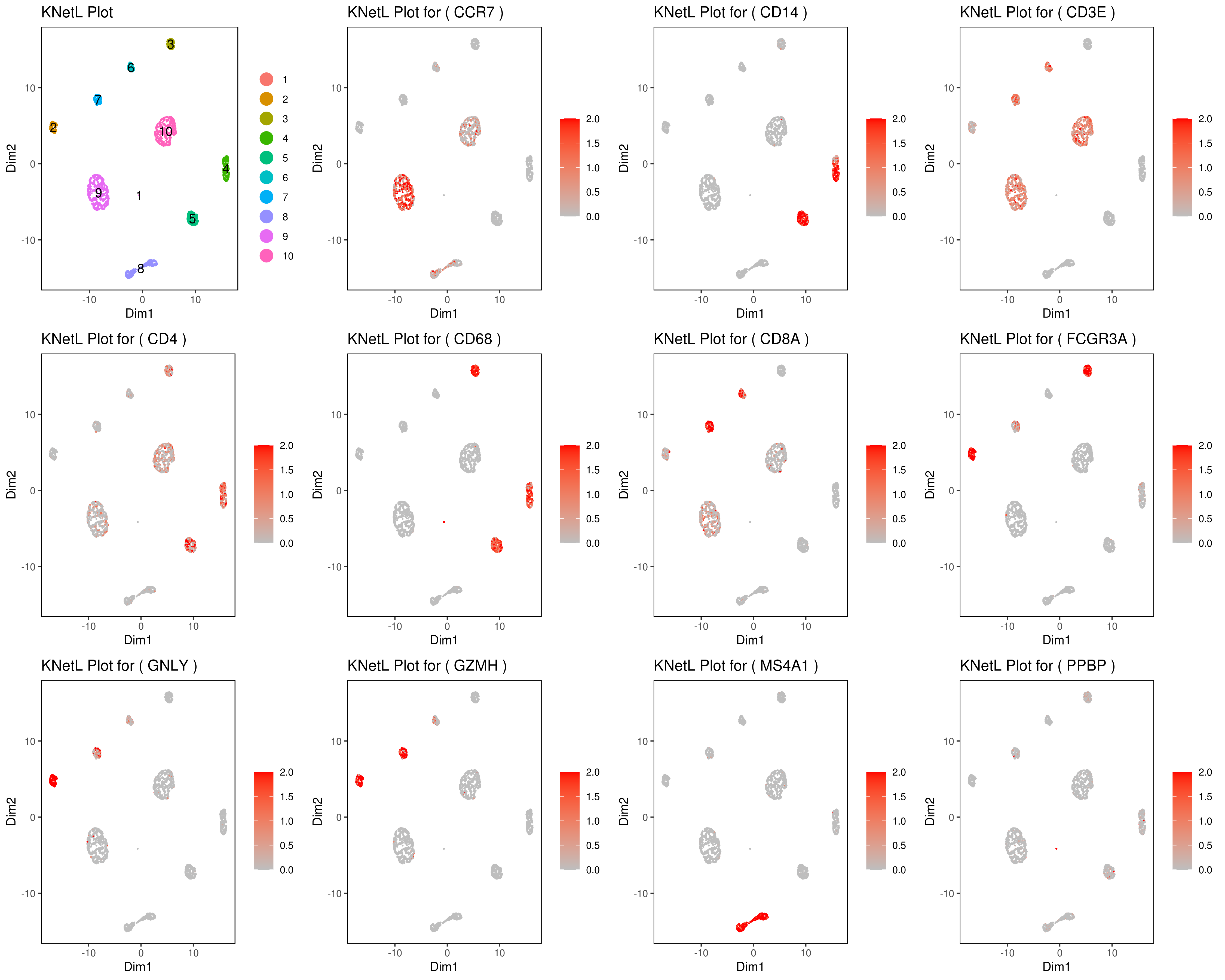
Multiple plots

Change the section in between #### signs for different plots (e.g. boxplot, bar, ...).

genelist = c("MS4A1","GNLY","FCGR3A","NKG7","CD14","CD3E","CD8A","CD4","GZMH","CCR7","CD68")

rm(list = ls(pattern="PL_")) for(i in genelist){ #### MyPlot <- gene.plot(my.obj, gene = i, interactive = F, cell.size = 0.1, plot.data.type = "knetl", data.type = "main", scaleValue = T, min.scale = 0,max.scale = 2.0, cell.transparency = 1) #### NameCol=paste("PL",i,sep="_") eval(call("<-", as.name(NameCol), MyPlot)) }

library(cowplot) filenames <- ls(pattern="PL_")

B <- cluster.plot(my.obj,plot.type = "knetl",interactive = F,cell.size = 0.1,cell.transparency = 1,anno.clust=T) filenames <- c("B",filenames)

png('genes_KNetL.png',width = 15, height = 12, units = 'in', res = 300) plot_grid(plotlist=mget(filenames)) dev.off()

or heatmap

heatmap.gg.plot(my.obj, gene = genelist, interactive = F, cluster.by = "clusters")

Make your own customized plots

You can export the data using this command (one or multiple genes):

gene.plot(my.obj, gene = "MS4A1", write.data = T, scaleValue = F, data.type = "main")

This would create a text file called "MS4A1.tsv".

head(read.table("MS4A1.tsv"))

V1 V2 Expression Clusters Conditions

#WT_AAACATACAACCAC.1 12.499481 -11.436633 0.000000 9 WT #WT_AAACATTGAGCTAC.1 -8.783793 24.417999 1.942233 8 WT #WT_AAACATTGATCAGC.1 -2.650761 10.932273 0.000000 10 WT #WT_AAACCGTGCTTCCG.1 -28.916702 -5.542731 0.000000 4 WT #WT_AAACCGTGTATGCG.1 21.211557 -31.626822 0.000000 2 WT #WT_AAACGCACTGGTAC.1 5.225419 -5.141192 0.000000 10 WT

you use this to make your own plots in ggplot2 or other visualization packages.

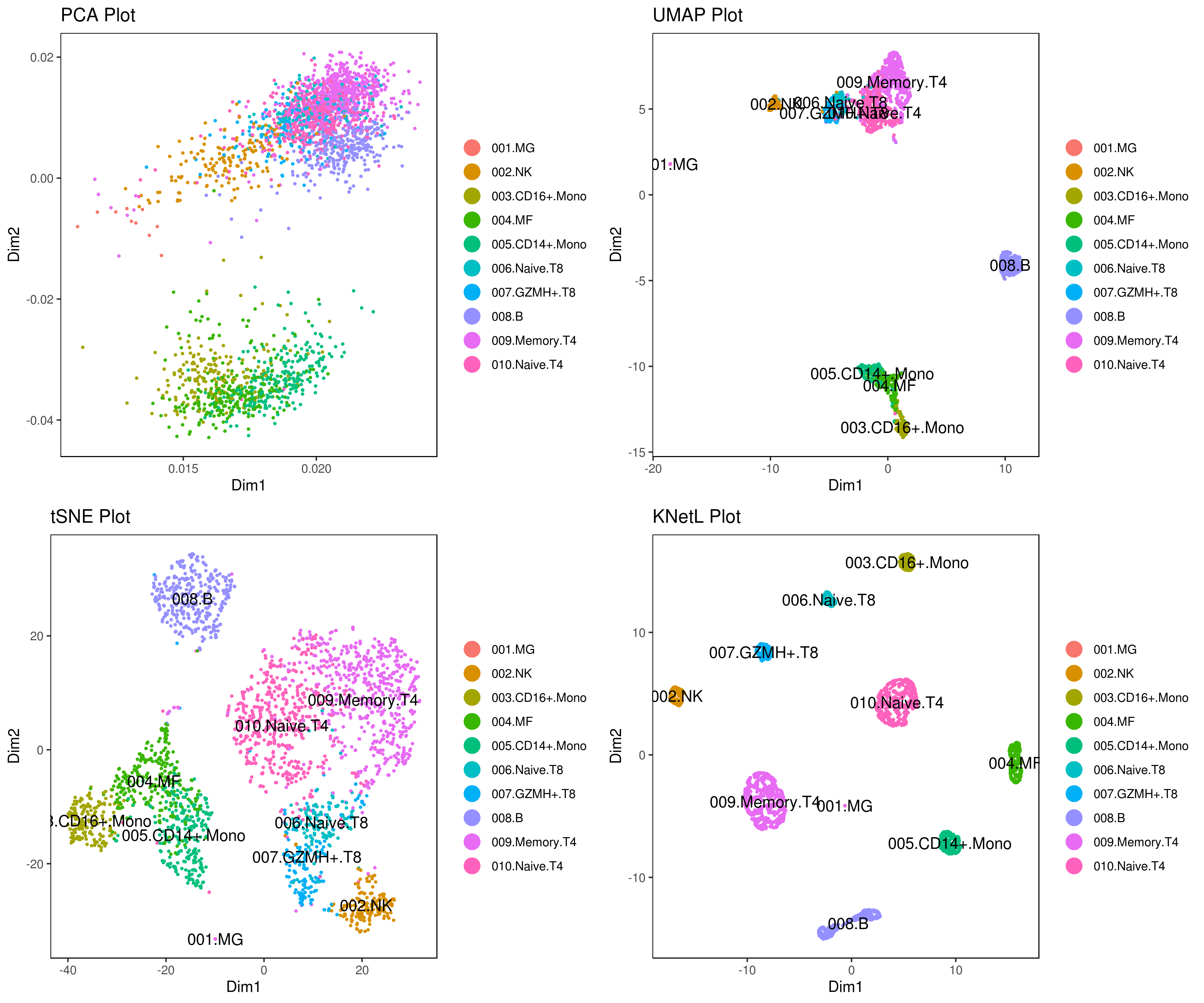
Annotating clusters

Labeling the clusters

#CD3E: only in T Cells #FCGR3A (CD16): in CD16+ monocytes and some expression NK cells #GNLY: NK cells #MS4A1: B cells #GZMH: in GZMH+ T8 cells and some expression NK cells #CD8A: in T8 cells #CD4: in T4 and some myeloid cells #CCR7: expressed more in memory cells #CD14: in CD14+ monocytes #CD68: in monocytes/MF

my.obj <- change.clust(my.obj, change.clust = 1, to.clust = "001.MG") my.obj <- change.clust(my.obj, change.clust = 2, to.clust = "002.NK") my.obj <- change.clust(my.obj, change.clust = 3, to.clust = "003.CD16+.Mono") my.obj <- change.clust(my.obj, change.clust = 4, to.clust = "004.MF") my.obj <- change.clust(my.obj, change.clust = 5, to.clust = "005.CD14+.Mono") my.obj <- change.clust(my.obj, change.clust = 6, to.clust = "006.Naive.T8") my.obj <- change.clust(my.obj, change.clust = 7, to.clust = "007.GZMH+.T8") my.obj <- change.clust(my.obj, change.clust = 8, to.clust = "008.B") my.obj <- change.clust(my.obj, change.clust = 9, to.clust = "009.Memory.T4") my.obj <- change.clust(my.obj, change.clust = 10, to.clust = "010.Naive.T4")

grid.arrange(A,B,C,D)

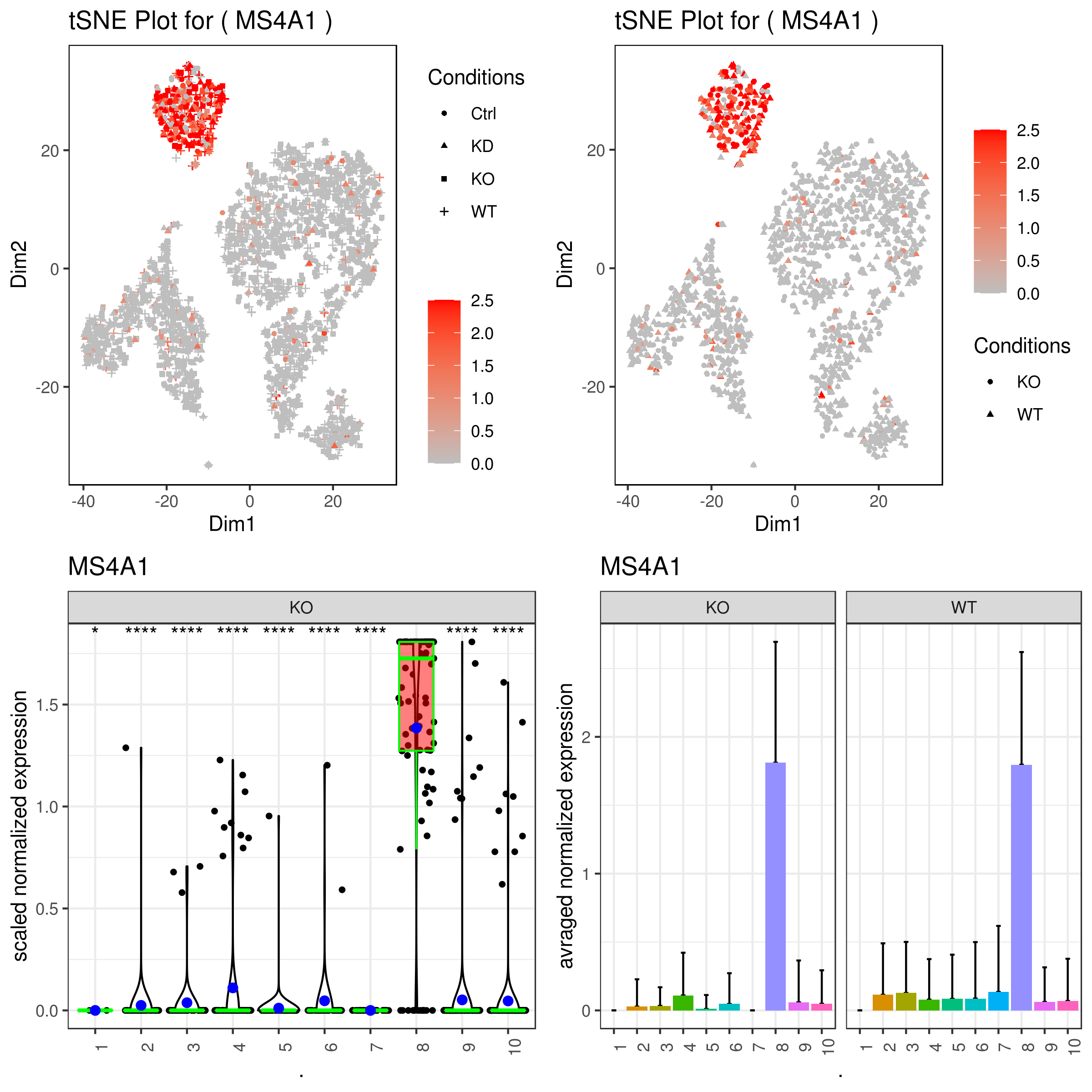
Plotting conditions and clusters for genes

A <- gene.plot(my.obj, gene = "MS4A1", plot.type = "scatterplot", interactive = F, cell.transparency = 1, scaleValue = TRUE, min.scale = 0, max.scale = 2.5, back.col = "white", cond.shape = TRUE) B <- gene.plot(my.obj, gene = "MS4A1", plot.type = "scatterplot", interactive = F, cell.transparency = 1, scaleValue = TRUE, min.scale = 0, max.scale = 2.5, back.col = "white", cond.shape = TRUE, conds.to.plot = c("KO","WT"))

C <- gene.plot(my.obj, gene = "MS4A1", plot.type = "boxplot", interactive = F, back.col = "white", cond.shape = TRUE, conds.to.plot = c("KO"))

D <- gene.plot(my.obj, gene = "MS4A1", plot.type = "barplot", interactive = F, cell.transparency = 1, back.col = "white", cond.shape = TRUE, conds.to.plot = c("KO","WT"))

library(gridExtra) grid.arrange(A,B,C,D)

Some example 2D and 3D plots and plotting clusters and conditions at the same time

example

cluster.plot(my.obj, cell.size = 1, plot.type = "umap", cell.color = "black", back.col = "white", col.by = "clusters", cell.transparency = 0.5, clust.dim = 2, cond.shape = T, interactive = T, out.name = "2d_UMAP_clusters_conds")

2D

cluster.plot(my.obj, cell.size = 1, plot.type = "tsne", cell.color = "black", back.col = "white", col.by = "clusters", cell.transparency = 0.5, clust.dim = 2, interactive = F)

interactive 2D

cluster.plot(my.obj, plot.type = "tsne", col.by = "clusters", clust.dim = 2, interactive = T, out.name = "tSNE_2D_clusters")

interactive 3D

cluster.plot(my.obj, plot.type = "tsne", col.by = "clusters", clust.dim = 3, interactive = T, out.name = "tSNE_3D_clusters")

Density plot for clusters

cluster.plot(my.obj, plot.type = "pca", col.by = "clusters", interactive = F, density=T)

Density plot for conditions

cluster.plot(my.obj, plot.type = "pca", col.by = "conditions", interactive = F, density=T)

cluster.plot(my.obj, cell.size = 1, plot.type = "diffusion", cell.color = "black", back.col = "white", col.by = "clusters", cell.transparency = 0.5, clust.dim = 2, interactive = F)

cluster.plot(my.obj, cell.size = 1, plot.type = "diffusion", cell.color = "black", back.col = "white", col.by = "clusters", cell.transparency = 0.5, clust.dim = 3, interactive = F)

To see the above made interactive plots click on these links: 2Dplot and 3Dplot

Differential Expression Analysis

The differential expression (DE) analysis function in iCellR allows the users to choose from any combinations of clusters and conditions. For example, a user with two samples (say WT and KO) has four different possible ways of comparisons:

a-Comparing a cluster/clusters with different cluster/clusters (e.g. cluster 1 and 2 vs. 4)

b-Comparing a cluster/clusters with different cluster/clusters only in one/more condition/conditions (e.g. cluster 1 vs cluster 2 but only the WT sample)

c-Comparing a condition/conditions with different condition/conditions (e.g. WT vs KO)

d-Comparing a condition/conditions with different condition/conditions only in one/more cluster/clusters (e.g. cluster 1 WT vs cluster 1 KO)

diff.res <- run.diff.exp(my.obj, de.by = "clusters", cond.1 = c(1,4), cond.2 = c(2)) diff.res1 <- as.data.frame(diff.res) diff.res1 <- subset(diff.res1, padj < 0.05) head(diff.res1)

baseMean 1_4 2 foldChange log2FoldChange pval

#AAK1 0.19554589 0.26338228 0.041792762 0.15867719 -2.655833 8.497012e-33 #ABHD14A 0.09645732 0.12708519 0.027038379 0.21275791 -2.232715 1.151865e-11 #ABHD14B 0.19132829 0.23177944 0.099644572 0.42991118 -1.217889 3.163623e-09 #ABLIM1 0.06901900 0.08749258 0.027148089 0.31029018 -1.688310 1.076382e-06 #AC013264.2 0.07383608 0.10584821 0.001279649 0.01208947 -6.370105 1.291674e-19 #AC092580.4 0.03730859 0.05112053 0.006003441 0.11743700 -3.090041 5.048838e-07 padj #AAK1 1.294690e-28 #ABHD14A 1.708446e-07 #ABHD14B 4.636290e-05 #ABLIM1 1.540087e-02 #AC013264.2 1.950557e-15 #AC092580.4 7.254675e-03

more examples

Comparing a condition/conditions with different condition/conditions (e.g. WT vs KO)

diff.res <- run.diff.exp(my.obj, de.by = "conditions", cond.1 = c("WT"), cond.2 = c("KO"))

Comparing a cluster/clusters with different cluster/clusters (e.g. cluster 1 and 2 vs. 4)

diff.res <- run.diff.exp(my.obj, de.by = "clusters", cond.1 = c(1,4), cond.2 = c(2))

Comparing a condition/conditions with different condition/conditions only in one/more cluster/clusters (e.g. cluster 1 WT vs cluster 1 KO)

diff.res <- run.diff.exp(my.obj, de.by = "clustBase.condComp", cond.1 = c("WT"), cond.2 = c("KO"), base.cond = 1)

Comparing a cluster/clusters with different cluster/clusters only in one/more condition/conditions (e.g. cluster 1 vs cluster 2 but only the WT sample)

diff.res <- run.diff.exp(my.obj, de.by = "condBase.clustComp", cond.1 = c(1), cond.2 = c(2), base.cond = "WT")

Volcano and MA plots

Volcano Plot

volcano.ma.plot(diff.res, sig.value = "pval", sig.line = 0.05, plot.type = "volcano", interactive = F)

MA Plot

volcano.ma.plot(diff.res, sig.value = "pval", sig.line = 0.05, plot.type = "ma", interactive = F)

Merging, resetting, renaming and removing clusters

let's say you want to merge cluster 3 and 2.

my.obj <- change.clust(my.obj, change.clust = 3, to.clust = 2)

to reset to the original clusters run this.

my.obj <- change.clust(my.obj, clust.reset = T)

you can also re-name the cluster numbers to cell types. Remember to reset after this so you can ran other analysis.

my.obj <- change.clust(my.obj, change.clust = 7, to.clust = "B Cell")

Let's say for what ever reason you want to remove acluster, to do so run this.

my.obj <- clust.rm(my.obj, clust.to.rm = 1)

Remember that this would perminantly remove the data from all the slots in the object except frrom raw.data slot in the object. If you want to reset you need to start from the filtering cells step in the biginging of the analysis (using cell.filter function).

To re-position the cells run tSNE again

my.obj <- run.tsne(my.obj, clust.method = "gene.model", gene.list = "my_model_genes.txt")

Use this for plotting as you make the changes

cluster.plot(my.obj, cell.size = 1, plot.type = "tsne", cell.color = "black", back.col = "white", col.by = "clusters", cell.transparency = 0.5, clust.dim = 2, interactive = F)

Cell gating

my.plot <- gene.plot(my.obj, gene = "GNLY", plot.type = "scatterplot", clust.dim = 2, interactive = F)

cell.gating(my.obj, my.plot = my.plot, plot.type = "tsne")

or

#my.plot <- cluster.plot(my.obj, # cell.size = 1, # cell.transparency = 0.5, # clust.dim = 2, # interactive = F)

After downloading the cell ids, use the following command to rename their cluster.

my.obj <- gate.to.clust(my.obj, my.gate = "cellGating.txt", to.clust = 10)

Batch correction (sample alignment) methods:

1- CPCA (iCellR)** recommended (faster than CCCA)

2- CCCA (iCellR)* recommended

3- MNN (scran wraper) optional

4- MultiCCA (Seurat wraper) optional

5- CPCA + KNetL based clustering (iCellR)*** recommended for best results!

1- How to perform Combined Principal Component Alignment (CPCA)

We analyzed nine PBMC sample datasets provided by the Broad Institute to detect batch differences. These datasets were generated using varying technologies, including 10x Chromium v2 (3 samples), 10x Chromium v3, CEL-Seq2, Drop-seq, inDrop, Seq-Well and SMART-Seq. For more info read:https://www.biorxiv.org/content/10.1101/2020.03.31.019109v1.full

download an object of 9 PBMC samples

sample.file.url = "https://genome.med.nyu.edu/results/external/iCellR/data/pbmc_data/my.obj.Robj"

download the file

download.file(url = sample.file.url, destfile = "my.obj.Robj", method = "auto")

load iCellR and the object

library(iCellR) load("my.obj.Robj")

run PCA on top 2000 genes

my.obj <- run.pca(my.obj, top.rank = 2000)

find best genes for second round PCA or batch alignment

my.obj <- find.dim.genes(my.obj, dims = 1:30,top.pos = 20, top.neg = 20) length(my.obj@gene.model)

########### Batch alignment (CPCA method)

my.obj <- iba(my.obj,dims = 1:30, k = 10,ba.method = "CPCA", method = "gene.model", gene.list = my.obj@gene.model)

impute data

my.obj <- run.impute(my.obj,dims = 1:10,data.type = "pca", nn = 10)

tSNE and UMAP

my.obj <- run.pc.tsne(my.obj, dims = 1:10) my.obj <- run.umap(my.obj, dims = 1:10)

save object

save(my.obj, file = "my.obj.Robj")

plot

library(gridExtra) A= cluster.plot(my.obj,plot.type = "umap",interactive = F,cell.size = 0.1) B= cluster.plot(my.obj,plot.type = "tsne",interactive = F,cell.size = 0.1) C= cluster.plot(my.obj,plot.type = "umap",col.by = "conditions",interactive = F,cell.size = 0.1) D=cluster.plot(my.obj,plot.type = "tsne",col.by = "conditions",interactive = F,cell.size = 0.1)

png('AllClusts.png', width = 12, height = 12, units = 'in', res = 300) grid.arrange(A,B,C,D) dev.off()

png('AllConds_clusts.png', width = 15, height = 15, units = 'in', res = 300) cluster.plot(my.obj, cell.size = 0.5, plot.type = "umap", cell.color = "black", back.col = "white", cell.transparency = 1, clust.dim = 2, interactive = F,cond.facet = T) dev.off()

genelist = c("PPBP","LYZ","MS4A1","GNLY","FCGR3A","NKG7","CD14","S100A9","CD3E","CD8A","CD4","CD19","IL7R","FOXP3","EPCAM")

for(i in genelist){ MyPlot <- gene.plot(my.obj, gene = i, interactive = F, conds.to.plot = NULL, cell.size = 0.1, data.type = "main", plot.data.type = "umap", scaleValue = T, min.scale = -2.5,max.scale = 2.0, cell.transparency = 1) NameCol=paste("PL",i,sep="_") eval(call("<-", as.name(NameCol), MyPlot)) }

UMAP = cluster.plot(my.obj,plot.type = "umap",interactive = F,cell.size = 0.1, anno.size=5) library(cowplot) filenames <- ls(pattern="PL_") filenames <- c("UMAP", filenames)

png('genes.png',width = 18, height = 15, units = 'in', res = 300) plot_grid(plotlist=mget(filenames)) dev.off()

2- How to perform Combined Coverage Correction Alignment (CCCA)

same as above only change the option to CCCA

my.obj <- iba(my.obj,dims = 1:30, k = 10,ba.method = "CCCA", method = "gene.model", gene.list = my.obj@gene.model)

3- How to perform mutual nearest neighbor (MNN) sample alignment

same as above only use run.mnn function instead of iba.

Run MNN

This would automatically run all the samples in your experiment

library(scran) my.obj <- run.mnn(my.obj, k=20, d=50, method = "gene.model", gene.list = my.obj@gene.model)

detach the scran pacakge after MNN as it masks some of the functions

detach("package:scran", unload=TRUE)

4- How to perform Seurat's MultiCCA sample alignment

same as above only use run.anchor function instead of iba.

Run Anchor

This would automatically run all the samples in your experiment

library(Seurat) my.obj <- run.anchor(my.obj, normalization.method = "SCT", scale.factor = 10000, selection.method = "vst", nfeatures = 2000, dims = 1:20)

5- How to perform CPCA + KNetL based clustering for sample alignment/integration

download an object of 9 PBMC samples

sample.file.url = "https://genome.med.nyu.edu/results/external/iCellR/example2/my.obj.Robj"

download the file

download.file(url = sample.file.url, destfile = "my.obj.Robj", method = "auto")

load iCellR and the object

library(iCellR) load("my.obj.Robj")

run PCA on top 2000 genes

my.obj <- run.pca(my.obj, top.rank = 2000)

find best genes for second round PCA or batch alignment

my.obj <- find.dim.genes(my.obj, dims = 1:30,top.pos = 20, top.neg = 20) length(my.obj@gene.model)

########### Batch alignment (CPCA method)

my.obj <- iba(my.obj,dims = 1:30, k = 10,ba.method = "CPCA", method = "gene.model", gene.list = my.obj@gene.model)

impute data

my.obj <- run.impute(my.obj,dims = 1:10,data.type = "pca", nn = 10)

tSNE and UMAP

my.obj <- run.pc.tsne(my.obj, dims = 1:10) my.obj <- run.umap(my.obj, dims = 1:10)

run KNetL

my.obj <- run.knetl(my.obj, dims = 1:20, k = 400)

cluster based on KNetL coordinates

The object is already clustered but here is an example:

my.obj <- iclust(my.obj, k = 300, data.type = "knetl")

save object

save(my.obj, file = "my.obj.Robj")

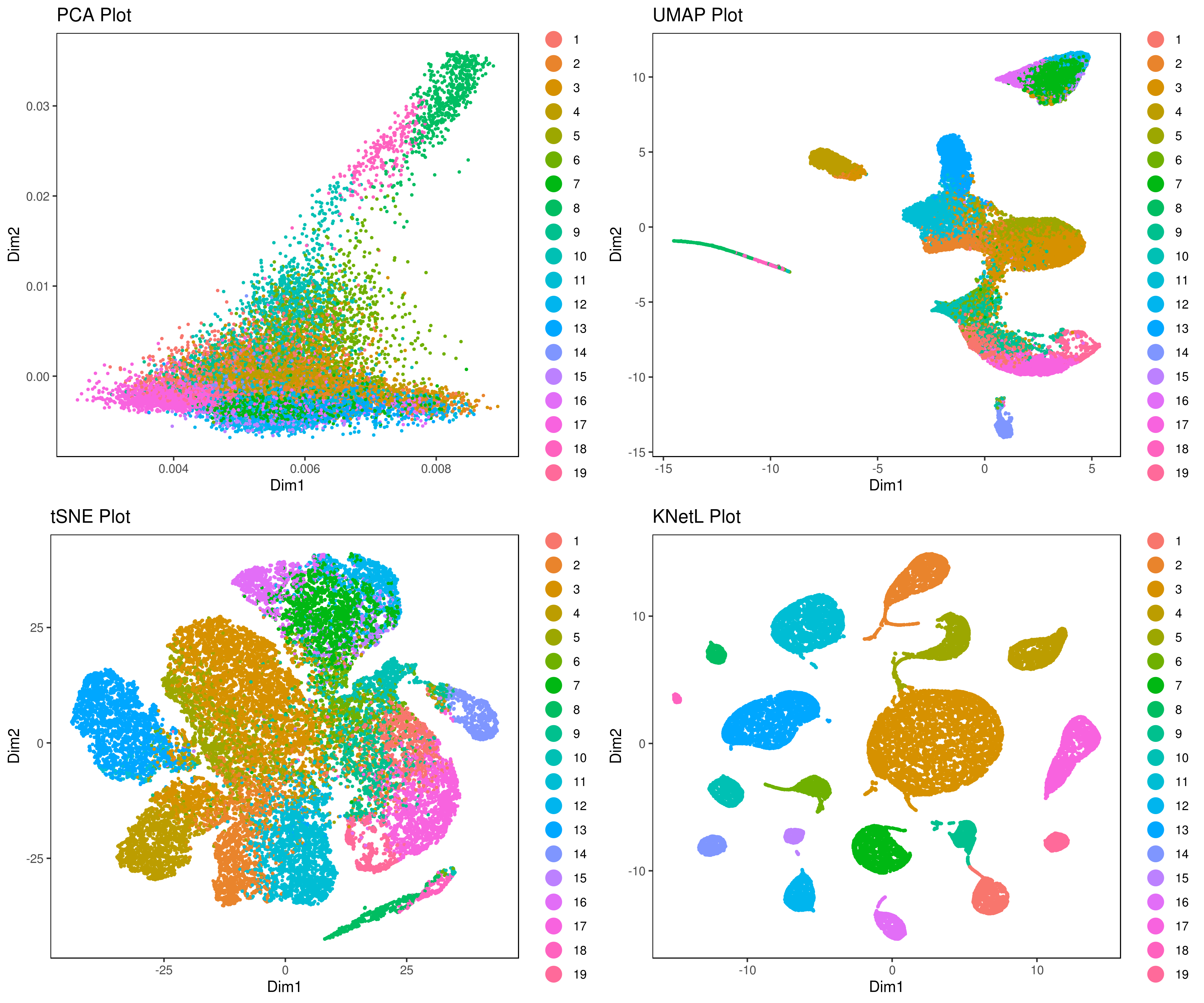
plot 1

A= cluster.plot(my.obj,plot.type = "pca",interactive = F,cell.size = 0.5,cell.transparency = 1, anno.clust=F) B= cluster.plot(my.obj,plot.type = "umap",interactive = F,cell.size = 0.5,cell.transparency = 1,anno.clust=F) C= cluster.plot(my.obj,plot.type = "tsne",interactive = F,cell.size = 0.5,cell.transparency = 1,anno.clust=F) D= cluster.plot(my.obj,plot.type = "knetl",interactive = F,cell.size = 0.5,cell.transparency = 1,anno.clust=F)

library(gridExtra) grid.arrange(A,B,C,D)

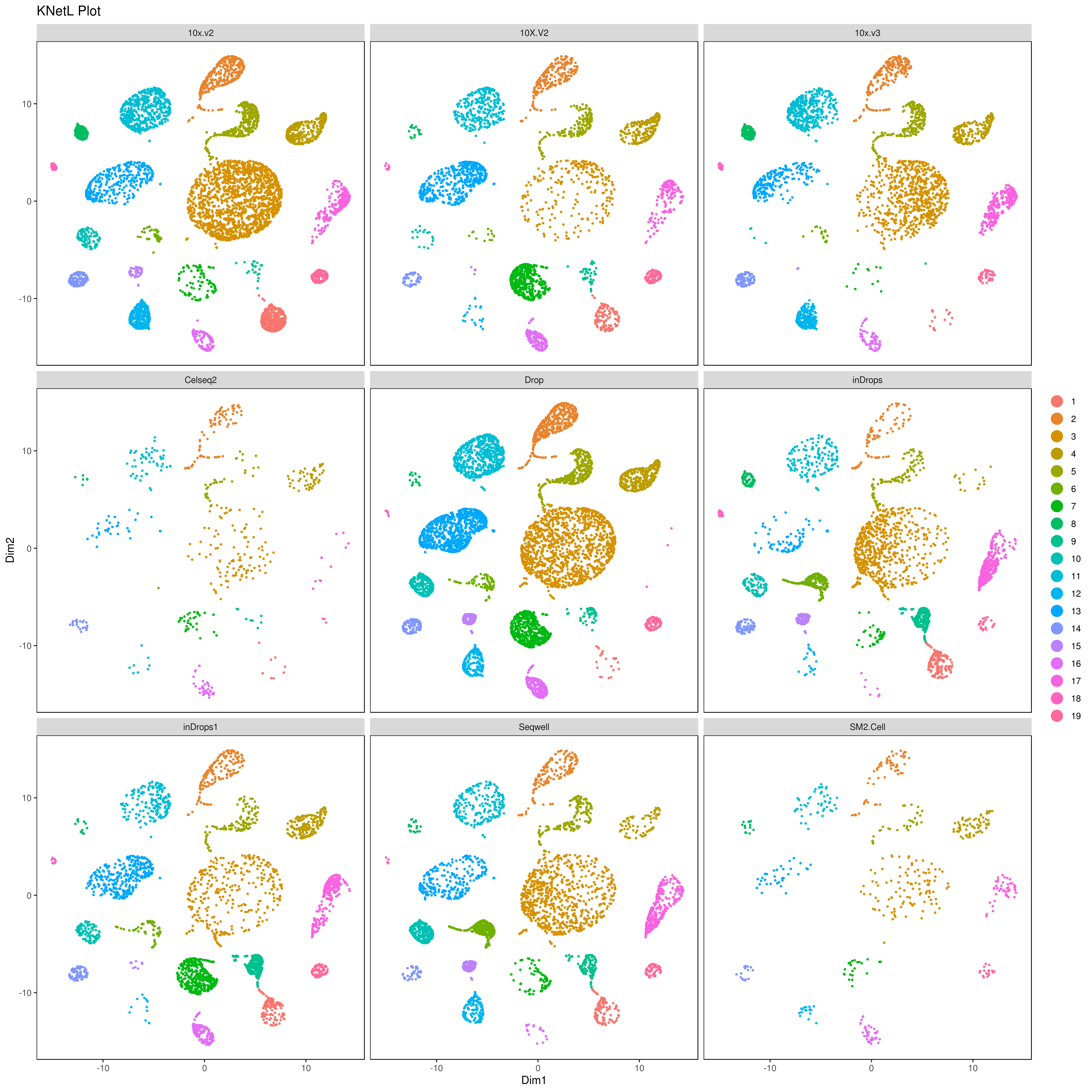
plot 2

cluster.plot(my.obj, cell.size = 0.5, plot.type = "knetl", cell.color = "black", back.col = "white", cell.transparency = 1, clust.dim = 2, interactive = F,cond.facet = T)

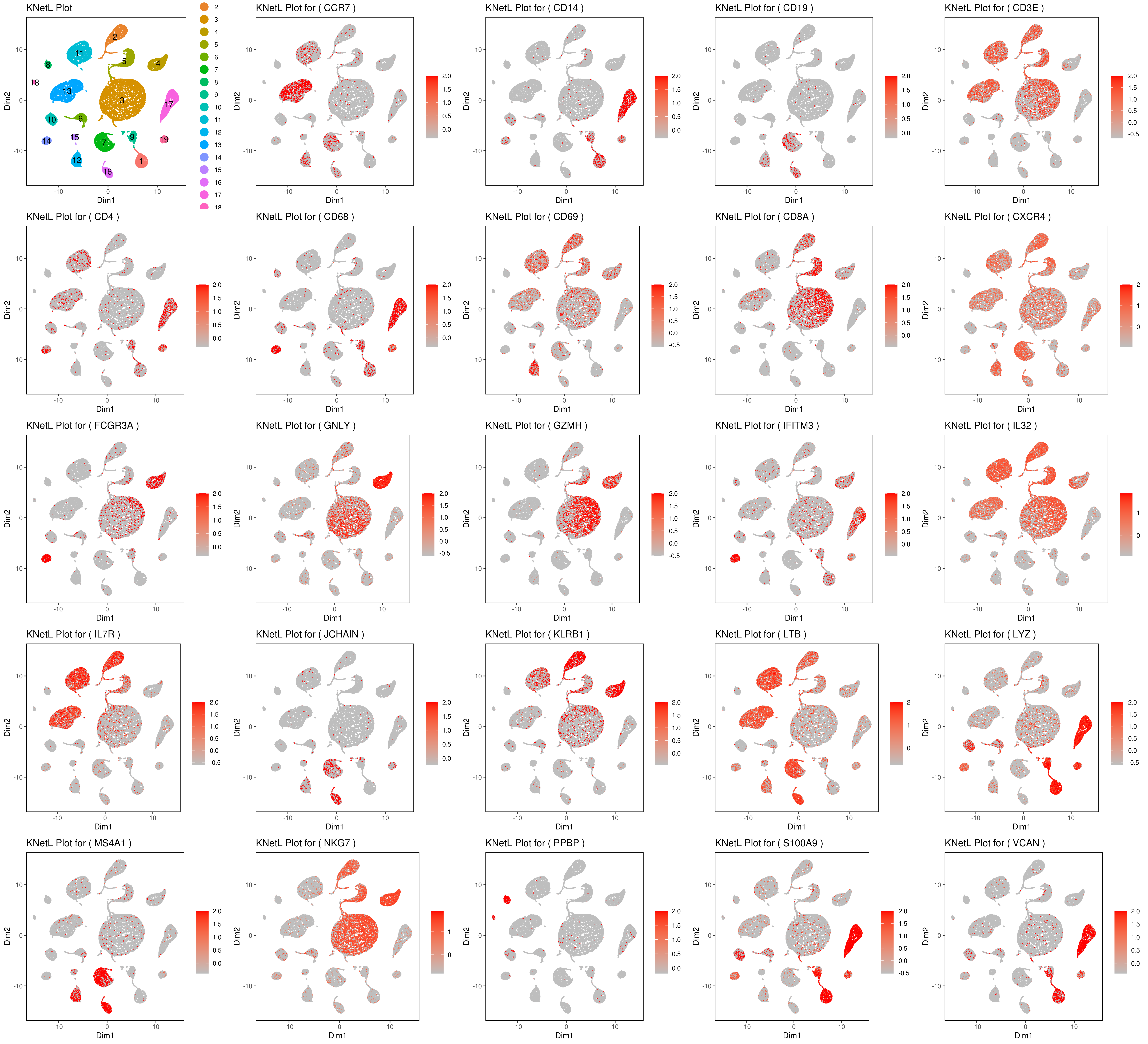
plot 3

genelist = c("LYZ","MS4A1","GNLY","FCGR3A","NKG7","CD14","S100A9","CD3E","CD8A","CD4","CD19","KLRB1","LTB","IL7R","GZMH","CD68","CCR7","CD68","CD69","CXCR4","IFITM3","IL32","JCHAIN","VCAN","PPBP")

rm(list = ls(pattern="PL_")) for(i in genelist){ MyPlot <- gene.plot(my.obj, gene = i, interactive = F, cell.size = 0.1, plot.data.type = "knetl", data.type = "main", scaleValue = T, min.scale = -2.5,max.scale = 2.0, cell.transparency = 1) NameCol=paste("PL",i,sep="_") eval(call("<-", as.name(NameCol), MyPlot)) }

library(cowplot) filenames <- ls(pattern="PL_")

B <- cluster.plot(my.obj,plot.type = "knetl",interactive = F,cell.size = 0.1,cell.transparency = 1,anno.clust=T) filenames <- c("B",filenames)

plot_grid(plotlist=mget(filenames))

Pseudotime analysis

MyGenes <- top.markers(marker.genes, topde = 50, min.base.mean = 0.2) MyGenes <- unique(MyGenes)

pseudotime.tree(my.obj, marker.genes = MyGenes, type = "unrooted", clust.method = "complete")

or

pseudotime.tree(my.obj, marker.genes = MyGenes, type = "classic", clust.method = "complete")

pseudotime.tree(my.obj, marker.genes = MyGenes, type = "jitter", clust.method = "complete")

Pseudotime analysis using monocle

library(monocle)

MyMTX <- my.obj@main.data GeneAnno <- as.data.frame(row.names(MyMTX)) colnames(GeneAnno) <- "gene_short_name" row.names(GeneAnno) <- GeneAnno$gene_short_name cell.cluster <- (my.obj@best.clust) Ha <- data.frame(do.call('rbind', strsplit(as.character(row.names(cell.cluster)),'_',fixed=TRUE)))[1] clusts <- paste("cl.",as.character(cell.cluster$clusters),sep="") cell.cluster <- cbind(cell.cluster,Ha,clusts) colnames(cell.cluster) <- c("Clusts","iCellR.Conds","iCellR.Clusts") Samp <- new("AnnotatedDataFrame", data = cell.cluster) Anno <- new("AnnotatedDataFrame", data = GeneAnno) my.monoc.obj <- newCellDataSet(as.matrix(MyMTX),phenoData = Samp, featureData = Anno)

find disperesedgenes

my.monoc.obj <- estimateSizeFactors(my.monoc.obj) my.monoc.obj <- estimateDispersions(my.monoc.obj) disp_table <- dispersionTable(my.monoc.obj)

unsup_clustering_genes <- subset(disp_table, mean_expression >= 0.1) my.monoc.obj <- setOrderingFilter(my.monoc.obj, unsup_clustering_genes$gene_id)

tSNE

my.monoc.obj <- reduceDimension(my.monoc.obj, max_components = 2, num_dim = 10,reduction_method = 'tSNE', verbose = T)

cluster

my.monoc.obj <- clusterCells(my.monoc.obj, num_clusters = 10)

plot conditions and clusters based on iCellR analysis

A <- plot_cell_clusters(my.monoc.obj, 1, 2, color = "iCellR.Conds") B <- plot_cell_clusters(my.monoc.obj, 1, 2, color = "iCellR.Clusts")

plot clusters based monocle analysis

C <- plot_cell_clusters(my.monoc.obj, 1, 2, color = "Cluster")

get marker genes from iCellR analysis

MyGenes <- top.markers(marker.genes, topde = 30, min.base.mean = 0.2) my.monoc.obj <- setOrderingFilter(my.monoc.obj, MyGenes)

my.monoc.obj <- reduceDimension(my.monoc.obj, max_components = 2,method = 'DDRTree')

order cells

my.monoc.obj <- orderCells(my.monoc.obj)

plot based on iCellR analysis and marker genes from iCellR

D <- plot_cell_trajectory(my.monoc.obj, color_by = "iCellR.Clusts")

heatmap genes from iCellR

plot_pseudotime_heatmap(my.monoc.obj[MyGenes,], cores = 1, cluster_rows = F, use_gene_short_name = T, show_rownames = T)

How to demultiplex with hashtag oligos (HTOs)

Read an example file

my.hto <- read.table(file = system.file('extdata', 'dense_umis.tsv', package = 'iCellR'), as.is = TRUE)

or

my.data <- load10x("filtered_feature_bc_matrix",gene.name = 2)

Your HTOs are usually in the end of all the gene names

tail(row.names(my.data),5)

[1] "TotalSeq.C0254_anti.human_Hashtag_4_Antibody"

[2] "TotalSeq.C0255_anti.human_Hashtag_5_Antibody"

[3] "TotalSeq.C0256_anti.human_Hashtag_6_Antibody"

[4] "TotalSeq.C0257_anti.human_Hashtag_7_Antibody"

[5] "TotalSeq.C0258_anti.human_Hashtag_8_Antibody"

your HTOs are usually in the matrix and have names that are different than gene names

Your HTO names

HTOs <- grep("^TotalSeq",row.names(my.data),value=T)

your gene names

RNAs <- subset(row.names(my.data), !(row.names(my.data) %in% HTOs))

MyHTOs <- subset(my.data, row.names(my.data) %in% HTOs) MyRNAs <- subset(my.data, row.names(my.data) %in% RNAs)

dim(MyHTOs) dim(MyRNAs)

run annotation

data <- hto.anno(hto.data = MyHTOs, cov.thr = 3, assignment.thr = 80) data <- (cbind(ID = rownames(data),data)) write.table((data),"HTOs_annotated_HSThigh.tsv",sep="\t", row.names =F)

head(data)

Hashtag1-GTCAACTCTTTAGCG Hashtag2-TGATGGCCTATTGGG

#TGACAACAGGGCTCTC 3 18 #AAGGAGCGTCATTAGC 7 24 #AGTGAGGAGACTGTAA 7 1761 #ATCCACCCATGTTCCC 753 20 #AAACGGGCAGGACCCT 728 24 #ATGTGTGAGTCTTGCA 4 25

Hashtag3-TTCCGCCTCTCTTTG Hashtag4-AGTAAGTTCAGCGTA

#TGACAACAGGGCTCTC 7 0 #AAGGAGCGTCATTAGC 8 0 #AGTGAGGAGACTGTAA 5 0 #ATCCACCCATGTTCCC 3 0 #AAACGGGCAGGACCCT 3 0 #ATGTGTGAGTCTTGCA 370 0

Hashtag5-AAGTATCGTTTCGCA Hashtag7-TGTCTTTCCTGCCAG unmapped

#TGACAACAGGGCTCTC 890 5 17 #AAGGAGCGTCATTAGC 2 3 3 #AGTGAGGAGACTGTAA 11 3 87 #ATCCACCCATGTTCCC 5 6 18 #AAACGGGCAGGACCCT 9 3 16 #ATGTGTGAGTCTTGCA 9 1011 25

assignment.annotation percent.match coverage low.cov

#TGACAACAGGGCTCTC Hashtag5-AAGTATCGTTTCGCA 94.68085 940 FALSE #AAGGAGCGTCATTAGC Hashtag2-TGATGGCCTATTGGG 51.06383 47 TRUE #AGTGAGGAGACTGTAA Hashtag2-TGATGGCCTATTGGG 93.97012 1874 FALSE #ATCCACCCATGTTCCC Hashtag1-GTCAACTCTTTAGCG 93.54037 805 FALSE #AAACGGGCAGGACCCT Hashtag1-GTCAACTCTTTAGCG 92.97573 783 FALSE #ATGTGTGAGTCTTGCA Hashtag7-TGTCTTTCCTGCCAG 70.01385 1444 FALSE

assignment.threshold

#TGACAACAGGGCTCTC good.assignment #AAGGAGCGTCATTAGC unsure #AGTGAGGAGACTGTAA good.assignment #ATCCACCCATGTTCCC good.assignment #AAACGGGCAGGACCCT good.assignment #ATGTGTGAGTCTTGCA unsure

plot

A = ggplot(data, aes(assignment.annotation,percent.match)) + geom_jitter(alpha = 0.25, color = "blue") + geom_boxplot(alpha = 0.5) + theme_bw() + theme(axis.text.x=element_text(angle=90))

B = ggplot(data, aes(low.cov,percent.match)) + geom_jitter(alpha = 0.25, color = "blue") + geom_boxplot(alpha = 0.5) + theme_bw() + theme(axis.text.x=element_text(angle=90))

library(gridExtra) Name="HTO_stats.png" png(Name, width = 8, height = 8, units = 'in', res = 300) grid.arrange(A,B,ncol=2) dev.off()

Filtering HTOs and merging the samples

let's see how many cells are there

dim(data)

let's say you want to have the cells that are above 80 % likelihood of belonging to an HTO

data <- subset(data, percent.match > 80)

let's see how many cells are left

dim(data)

Take the HTO IDs that passed filtering

bestHTOs <- as.character(unique(data$assignment.annotation))

####################

create new files (matrices) for each HTO (with number of cells added to the folder names)

####################

library(Matrix) for(i in bestHTOs){ sample <- row.names(subset(data,data$assignment.annotation == i)) message(paste(" getting sample",i,"...")) sample <- MyRNAs[ , which(names(MyRNAs) %in% sample)] message(paste(" number of cells",dim(sample)[2])) Name=paste("RNAs",i,dim(sample)[2],sep="_") message(paste(" writing sample",i,"...")) dir.create(Name) COLs <- colnames(sample) ROWs <- row.names(sample) colnames(sample) <- NULL row.names(sample) <- NULL sparse.gbm <- Matrix(as.matrix.data.frame(sample), sparse = T ) Name1=paste(Name,"matrix.mtx",sep="/") writeMM(obj = sparse.gbm, file=Name1) Name1=paste(Name,"barcodes.tsv.gz",sep="/") write.table((COLs),gzfile(Name1), row.names =FALSE, quote = FALSE, col.names = FALSE) MY.ROWs <- cbind(ROWs,ROWs) Name1=paste(Name,"genes.tsv.gz",sep="/") write.table((MY.ROWs),gzfile(Name1),sep="\t", row.names =F, quote = FALSE, col.names = FALSE) }

#################### ####################

example data aggregation for 2 samples/HTOs

my.data <- data.aggregation(samples = c("HTO1","HTO2"), condition.names = c("HTO1","HTO2"))

make iCellR object

my.obj <- make.obj(my.data)

The rest is as above :)

How to use i.score to rank/score the cells:

This data is from this publication (GEO number: GSE156246 and PMID: 34911733)

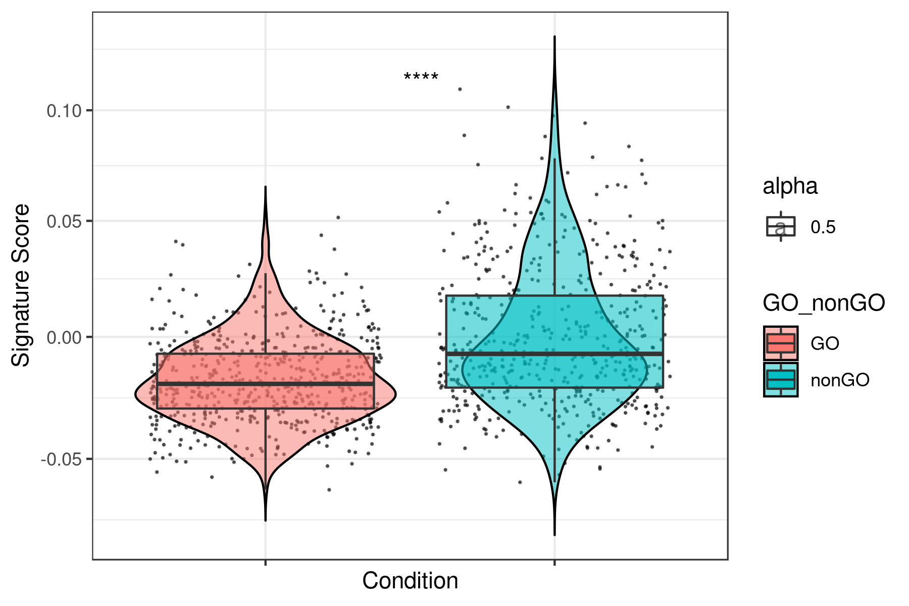
This is a how to guide to run i.score function in iCellR and to reproduce the above published data for G0 and non G0 cells.

Download the sample iCellR objects (used in the publication) from here: https://genome.med.nyu.edu/results/external/iCellR/i.score/(my.obj@raw.data in these objects are log normalized)

Download sample gene signatures from here: https://genome.med.nyu.edu/results/external/iCellR/i.score/gene_signatures.tar.gz(gene signatures used in the publication are in the supplementary data of the paper)

load sample gene signature that are in iCellR

(these cell cycle signatures are from here: https://www.nature.com/articles/s41586-019-1884-x)

library(iCellR) G0 <- readLines(system.file('extdata', 'G0.txt', package = 'iCellR')) G1S <- readLines(system.file('extdata', 'G1S.txt', package = 'iCellR')) G2M <- readLines(system.file('extdata', 'G2M.txt', package = 'iCellR')) M <- readLines(system.file('extdata', 'M.txt', package = 'iCellR')) MG1 <- readLines(system.file('extdata', 'MG1.txt', package = 'iCellR')) S <- readLines(system.file('extdata', 'S.txt', package = 'iCellR'))

load all the gene signatures

Melnick_10_GILMORE_CORE_NFKB_PATHWAY.txt <- readLines("10_GILMORE_CORE_NFKB_PATHWAY.txt") Melnick_11_HALLMARK_MYC_TARGETS_V1.txt <- readLines("11_HALLMARK_MYC_TARGETS_V1.txt") Melnick_12_GO_BETA_CATENIN_BINDING.txt <- readLines("12_GO_BETA_CATENIN_BINDING.txt") Melnick_13_PID_BETA_CATENIN_NUC_PATHWAY.txt <- readLines("13_PID_BETA_CATENIN_NUC_PATHWAY.txt") Melnick_14_PID_WNT_SIGNALING_PATHWAY.txt <- readLines("14_PID_WNT_SIGNALING_PATHWAY.txt") Melnick_15_PID_WNT_CANONICAL_PATHWAY.txt <- readLines("15_PID_WNT_CANONICAL_PATHWAY.txt") Melnick_16_Pribluda_SENESCENCE_INFLAMMATORY_GENES.txt <- readLines("16_Pribluda_SENESCENCE_INFLAMMATORY_GENES.txt") Melnick_17_FRIDMAN_SENESCENCE_DN.txt <- readLines("17_FRIDMAN_SENESCENCE_DN.txt") Melnick_18_FRIDMAN_SENESCENCE_UP.txt <- readLines("18_FRIDMAN_SENESCENCE_UP.txt") Melnick_19_DeJONGE_LSC_TOP50_genes.txt <- readLines("19_DeJONGE_LSC_TOP50_genes.txt") Melnick_1_AML1566_AraC_UP.txt <- readLines("1_AML1566_AraC_UP.txt") Melnick_20_GAL_LEUKEMIC_STEM_CELL_UP.txt <- readLines("20_GAL_LEUKEMIC_STEM_CELL_UP.txt") Melnick_21_GAL_LEUKEMIC_STEM_CELL_DN.txt <- readLines("21_GAL_LEUKEMIC_STEM_CELL_DN.txt") Melnick_22_EPPERT_CE_HSC_LSC.txt <- readLines("22_EPPERT_CE_HSC_LSC.txt") Melnick_23_JAATINEN_HEMATOPOIETIC_STEM_CELL_UP.txt <- readLines("23_JAATINEN_HEMATOPOIETIC_STEM_CELL_UP.txt") Melnick_24_JAATINEN_HEMATOPOIETIC_STEM_CELL_DN.txt <- readLines("24_JAATINEN_HEMATOPOIETIC_STEM_CELL_DN.txt") Melnick_25_INFLAMMATORY_RESPONSE.txt <- readLines("25_INFLAMMATORY_RESPONSE.txt") Melnick_26_RAMALHO_STEMNESS_DN.txt <- readLines("26_RAMALHO_STEMNESS_DN.txt") Melnick_27_RAMALHO_STEMNESS_UP.txt <- readLines("27_RAMALHO_STEMNESS_UP.txt") Melnick_28_REACTOME_REGULATION_OF_MITOTIC_CELL_CYCLE.txt <- readLines("28_REACTOME_REGULATION_OF_MITOTIC_CELL_CYCLE.txt") Melnick_2_AML1566_AraC_DN.txt <- readLines("2_AML1566_AraC_DN.txt") Melnick_3_DUY_CISG_UP.txt <- readLines("3_DUY_CISG_UP.txt") Melnick_4_DUY_CISG_DN.txt <- readLines("4_DUY_CISG_DN.txt") Melnick_5_DIAPAUSE_UP_BOROVIAK.txt <- readLines("5_DIAPAUSE_UP_BOROVIAK.txt") Melnick_6_BOROVIAK_DIAPAUSE_DN.txt <- readLines("6_BOROVIAK_DIAPAUSE_DN.txt") Melnick_7_SASP_COPPE.txt <- readLines("7_SASP_COPPE.txt") Melnick_8_SALDIVAR_ATR_SUPPRESSED_TARGETS.txt <- readLines("8_SALDIVAR_ATR_SUPPRESSED_TARGETS.txt") Melnick_9_BIOCARTA_NFKB_PATHWAY.txt <- readLines("9_BIOCARTA_NFKB_PATHWAY.txt") diapause_neg.txt <- readLines("diapause_neg.txt") diapause_pos_and_neg.txt <- readLines("diapause_pos_and_neg.txt") diapause_pos.txt <- readLines("diapause_pos.txt") DTP_sig_150_Down.txt <- readLines("DTP_sig_150_Down.txt") DTP_sig_150_up.txt <- readLines("DTP_sig_150_up.txt") Lum_uniq_down.txt <- readLines("Lum_uniq_down.txt") Lum_uniq_up.txt <- readLines("Lum_uniq_up.txt") Mes_uniq_down.txt <- readLines("Mes_uniq_down.txt") Mes_uniq_up.txt <- readLines("Mes_uniq_up.txt") panDTP_DN.txt <- readLines("new_panDTP_DN.txt") panDTP_up.txt <- readLines("new_panDTP_up.txt") mes_DTP_included_DEG_DN.txt <- readLines("new_mes_DTP_included_DEG_DN.txt") mes_DTP_included_DEG_UP.txt <- readLines("new_mes_DTP_included_DEG_UP.txt") lum_DTP_included_DEG_DN.txt <- readLines("new_lum_DTP_included_DEG_DN.txt") lum_DTP_included_DEG_UP.txt <- readLines("new_lum_DTP_included_DEG_UP.txt") lum_DTP_specific_UP_noCC.txt <- readLines("new_lum_DTP_specific_UP_noCC_.txt") mes_DTP_specific_UP_noCC.txt <- readLines("new_mes_DTP_specific_UP_noCC_.txt")

Group all the signatures in one character object:

All <- c("Melnick_10_GILMORE_CORE_NFKB_PATHWAY.txt","Melnick_11_HALLMARK_MYC_TARGETS_V1.txt","Melnick_12_GO_BETA_CATENIN_BINDING.txt","Melnick_13_PID_BETA_CATENIN_NUC_PATHWAY.txt","Melnick_14_PID_WNT_SIGNALING_PATHWAY.txt","Melnick_15_PID_WNT_CANONICAL_PATHWAY.txt","Melnick_16_Pribluda_SENESCENCE_INFLAMMATORY_GENES.txt","Melnick_17_FRIDMAN_SENESCENCE_DN.txt","Melnick_18_FRIDMAN_SENESCENCE_UP.txt","Melnick_19_DeJONGE_LSC_TOP50_genes.txt","Melnick_1_AML1566_AraC_UP.txt","Melnick_20_GAL_LEUKEMIC_STEM_CELL_UP.txt","Melnick_21_GAL_LEUKEMIC_STEM_CELL_DN.txt","Melnick_22_EPPERT_CE_HSC_LSC.txt","Melnick_23_JAATINEN_HEMATOPOIETIC_STEM_CELL_UP.txt","Melnick_24_JAATINEN_HEMATOPOIETIC_STEM_CELL_DN.txt","Melnick_25_INFLAMMATORY_RESPONSE.txt","Melnick_26_RAMALHO_STEMNESS_DN.txt","Melnick_27_RAMALHO_STEMNESS_UP.txt","Melnick_28_REACTOME_REGULATION_OF_MITOTIC_CELL_CYCLE.txt","Melnick_2_AML1566_AraC_DN.txt","Melnick_3_DUY_CISG_UP.txt","Melnick_4_DUY_CISG_DN.txt","Melnick_5_DIAPAUSE_UP_BOROVIAK.txt","Melnick_6_BOROVIAK_DIAPAUSE_DN.txt","Melnick_7_SASP_COPPE.txt","Melnick_8_SALDIVAR_ATR_SUPPRESSED_TARGETS.txt","Melnick_9_BIOCARTA_NFKB_PATHWAY.txt","diapause_neg.txt","diapause_pos_and_neg.txt","diapause_pos.txt","DTP_sig_150_Down.txt","DTP_sig_150_up.txt","Lum_uniq_down.txt","Lum_uniq_up.txt","Mes_uniq_down.txt","Mes_uniq_up.txt","G0","G1S","G2M","M","MG1","S","panDTP_DN.txt","panDTP_up.txt","mes_DTP_included_DEG_DN.txt","mes_DTP_included_DEG_UP.txt","lum_DTP_included_DEG_DN.txt","lum_DTP_included_DEG_UP.txt","lum_DTP_specific_UP_noCC.txt","mes_DTP_specific_UP_noCC.txt")

Load your sample iCellR object

Score for cell cycle gene signatures with any of the following scoring methods: tirosh, mean, sum, gsva, ssgsea, zscore and plage. (tirosh and zscore methods are recommended to perform best)

dat1 <- i.score(my.obj, scoring.List = c("G0","G1S","G2M","M","MG1","S") ,scoring.method = "tirosh",return.stats = TRUE, data.type = "raw.data") write.table(dat1,"tirosh_G0.tsv",sep="\t")

Score for all the other signatures (tirosh, mean, sum, gsva, ssgsea, zscore and plage)

dat2 <- i.score(my.obj, scoring.List = All ,scoring.method = "tirosh",return.stats = TRUE, data.type = "raw.data") write.table(dat2,"tirosh_all.tsv",sep="\t")

Prepare data to plot (marge dat1 and dat2)

dir.create("boxplots_tirosh") setwd("boxplots_tirosh")

data <- read.table("../tirosh_all.tsv",sep="\t",header=T) dataCC <- read.table("../tirosh_G0.tsv",sep="\t",header=T)

df = as.character(dataCC$assignment.annotation) == "G0" df[ df == "TRUE" ] <- "GO" df[ df == "FALSE" ] <- "nonGO"

data <- cbind(cond = rep("sample",length(df)), ID = rownames(data), assignment.annotation = dataCC$assignment.annotation, GO_nonGO = df, data)

write.table((data),file="data.xls",sep="\t", row.names =F)

Plot all the signatures individually:

data <- read.table("data.xls",sep="\t",header=T)

g <- head(data)[5:55] g <- colnames(g)

library(ggpubr)

for(i in g){ name <- paste("boxplot_",i,".png",sep="") png(name,width = 6, height = 4, units = 'in', res = 300) print(ggplot(data, aes(x= GO_nonGO,y=data[, i],fill = GO_nonGO, alpha = 0.5)) + geom_jitter(size = 0.2, color="black") + geom_violin(trim=FALSE, col = "black", alpha = 0.5) + geom_boxplot(outlier.color = NA) + theme_bw() + xlab("Condition") + ylab("Signature Score") + scale_y_continuous(trans = "log1p") + stat_compare_means(aes(group = GO_nonGO), label = "p.signif", label.x = 1.5) + theme(axis.text.x = element_blank())) dev.off() }

Example for "lum_DTP_included_DEG_DN.txt"

To see all the plots made as above go to this link:https://genome.med.nyu.edu/results/external/iCellR/i.score/test/boxplots_tirosh/

How to analyze CITE-seq data using iCellR

Download test samples

sample.file.url = "https://genome.med.nyu.edu/results/external/iCellR/data/CITE-Seq_sample_RNA.tsv.gz"

download RNA file

download.file(url = sample.file.url, destfile = "CITE-Seq_sample_RNA.tsv.gz", method = "auto")

sample.file.url = "https://genome.med.nyu.edu/results/external/iCellR/data/CITE-Seq_sample_ADT.tsv.gz"

download ADT file

download.file(url = sample.file.url, destfile = "CITE-Seq_sample_ADT.tsv.gz", method = "auto")

Read the files and make your object

Read RNA file

rna.data <- read.delim("CITE-Seq_sample_RNA.tsv.gz",header=TRUE)

see the head

head(rna.data)[1:3]

CTGTTTACACCGCTAG CTCTACGGTGTGGCTC AGCAGCCAGGCTCATT

#A1BG 0 0 0 #A1BG-AS1 0 0 0 #A1CF 0 0 0 #A2M 0 0 0 #A2M-AS1 0 0 0 #A2ML1 0 0 0

Read ADT file

adt.data <- read.delim("CITE-Seq_sample_ADT.tsv.gz",header=TRUE)

see the head

head(adt.data)[1:3]

CTGTTTACACCGCTAG CTCTACGGTGTGGCTC AGCAGCCAGGCTCATT

#CD3 60 52 89 #CD4 72 49 112 #CD8 76 59 61 #CD45RA 575 3943 682 #CD56 64 68 87 #CD16 161 107 117

if you had multiple sample use the data.aggregation function for both RNA and ADT data.

make iCellR object

my.obj <- make.obj(rna.data)

check object

my.obj ################################### ,--. ,-----. ,--.,--.,------. --'' .--./ ,---. | || || .--. ' ,--.| | | .-. :| || || '--'.' | |' '--'\ --. | || || | --' -----' ----'--'--'`--' '--' ################################### An object of class iCellR version: 1.1.4 Raw/original data dimentions (rows,columns): 20501,8617 Data conditions: no conditions/single sample Row names: A1BG,A1BG-AS1,A1CF ... Columns names: CTGTTTACACCGCTAG,CTCTACGGTGTGGCTC,AGCAGCCAGGCTCATT ... ################################### QC stats performed:FALSE, PCA performed:FALSE, CCA performed:FALSE Clustering performed:FALSE, Number of clusters:0 tSNE performed:FALSE, UMAP performed:FALSE, DiffMap performed:FALSE Main data dimentions (rows,columns):0,0 Normalization factors:,... Imputed data dimentions (rows,columns):0,0 ############## scVDJ-Seq ########### VDJ data dimentions (rows,columns):0,0 ############## CITE-Seq ############ ADT raw data dimentions (rows,columns):0,0 ADT main data dimentions (rows,columns):0,0 ADT columns names:... ADT row names:... ########### iCellR object ##########

add ADT data

my.obj <- add.adt(my.obj, adt.data = adt.data)

check too see

ADT raw data dimentions (rows,columns):10,8617 ADT main data dimentions (rows,columns):0,0 ADT columns names:... ADT row names:...

########### iCellR object ##########

QC, filter, normalize, merge ADT and RNA data, run PCA and UMAP

QC

my.obj <- qc.stats(my.obj, s.phase.genes = s.phase, g2m.phase.genes = g2m.phase)

plot as mentioned above

filter

my.obj <- cell.filter(my.obj, min.mito = 0, max.mito = 0.07 , min.genes = 500, max.genes = 4000, min.umis = 0, max.umis = Inf)

normalize RNA

my.obj <- norm.data(my.obj, norm.method = "ranked.glsf", top.rank = 500)

normalize ADT

my.obj <- norm.adt(my.obj)

gene stats

my.obj <- gene.stats(my.obj, which.data = "main.data")

find genes for PCA

my.obj <- make.gene.model(my.obj, my.out.put = "data", dispersion.limit = 1.5, base.mean.rank = 500, no.mito.model = T, mark.mito = T, interactive = F, no.cell.cycle = T, out.name = "gene.model")

merge RNA and ADT data

my.obj <- adt.rna.merge(my.obj, adt.data = "main")

run PCA and the rest is as above

my.obj <- run.pca(my.obj, method = "gene.model", gene.list = my.obj@gene.model,data.type = "main")

2 pass PCA

my.obj <- find.dim.genes(my.obj, dims = 1:20,top.pos = 20, top.neg = 20)

second round PC

my.obj <- run.pca(my.obj, method = "gene.model", gene.list = my.obj@gene.model,data.type = "main")

my.obj <- run.umap(my.obj, dims = 1:10)

check your object

my.obj ################################### ,--. ,-----. ,--.,--.,------. --'' .--./ ,---. | || || .--. ' ,--.| | | .-. :| || || '--'.' | |' '--'\ --. | || || | --' -----' ----'--'--'`--' '--' ################################### An object of class iCellR version: 1.1.4 Raw/original data dimentions (rows,columns): 20501,8617 Data conditions: no conditions/single sample Row names: A1BG,A1BG-AS1,A1CF ... Columns names: CTGTTTACACCGCTAG,CTCTACGGTGTGGCTC,AGCAGCCAGGCTCATT ... ################################### QC stats performed:TRUE, PCA performed:TRUE, CCA performed:FALSE Clustering performed:TRUE, Number of clusters:14 tSNE performed:FALSE, UMAP performed:TRUE, DiffMap performed:FALSE Main data dimentions (rows,columns):20511,8305 Normalization factors:8.448547776071,... Imputed data dimentions (rows,columns):0,0 ############## scVDJ-Seq ########### VDJ data dimentions (rows,columns):0,0 ############## CITE-Seq ############ ADT raw data dimentions (rows,columns):10,8617 ADT main data dimentions (rows,columns):10,8617 ADT columns names:CTGTTTACACCGCTAG... ADT row names:ADT_CD3... ########### iCellR object ##########

plot

find ADT gene names

grep("^ADT_", rownames(my.obj@main.data),value=T)

[1] "ADT_CD3" "ADT_CD4" "ADT_CD8" "ADT_CD45RA" "ADT_CD56"

[6] "ADT_CD16" "ADT_CD11c" "ADT_CD14" "ADT_CD19" "ADT_CD34"

A = gene.plot(my.obj, gene = "ADT_CD3", plot.data.type = "umap", interactive = F, cell.transparency = 0.5)

B = gene.plot(my.obj, gene = "CD3E", plot.data.type = "umap", interactive = F, cell.transparency = 0.5)

C = gene.plot(my.obj, gene = "ADT_CD16", plot.data.type = "umap", interactive = F, cell.transparency = 0.5)

D = gene.plot(my.obj, gene = "FCGR3A", plot.data.type = "umap", interactive = F, cell.transparency = 0.5)

library(gridExtra) grid.arrange(A,B,C,D)

How to analyze scVDJ-seq data using iCellR

Here is an example of how to add VDJ data.

an example file

my.vdj <- read.csv(file = system.file('extdata', 'all_contig_annotations.csv', package = 'iCellR'), as.is = TRUE)

head(my.vdj)

barcode is_cell contig_id high_confidence length

#1 AAACCTGTCCGAACGC-1 True AAACCTGTCCGAACGC-1_contig_1 True 654 #2 AAACCTGTCCGAACGC-1 True AAACCTGTCCGAACGC-1_contig_2 True 697 #3 AAACCTGTCCGAACGC-1 True AAACCTGTCCGAACGC-1_contig_3 False 496 #4 AAACCTGTCCGAACGC-1 True AAACCTGTCCGAACGC-1_contig_4 True 539 #5 AAACCTGTCGATGAGG-1 True AAACCTGTCGATGAGG-1_contig_1 True 705 #6 AAACCTGTCGATGAGG-1 True AAACCTGTCGATGAGG-1_contig_2 True 491

chain v_gene d_gene j_gene c_gene full_length productive cdr3

#1 TRB TRBV4-1 None TRBJ2-7 TRBC2 True True CASSQGVEQYF #2 TRA TRAV8-1 None TRAJ42 TRAC True True CAVKGGSQGNLIF #3 TRB None None TRBJ1-4 TRBC1 False None None #4 Multi None None TRAJ10 TRBC1 False None None #5 TRB TRBV5-5 TRBD1 TRBJ2-7 TRBC1 True True CASSLVSGGNEQYF #6 TRB None None TRBJ1-2 TRBC1 False None None

cdr3_nt reads umis raw_clonotype_id

#1 TGCGCCAGCAGCCAAGGGGTCGAGCAGTACTTC 42610 19 clonotype150 #2 TGTGCCGTGAAGGGAGGAAGCCAAGGAAATCTCATCTTT 12297 4 clonotype150 #3 None 4314 1 clonotype150 #4 None 2212 1 clonotype150 #5 TGTGCCAGCAGCTTGGTCTCAGGGGGAAACGAGCAGTACTTC 21148 8 clonotype2 #6 None 17717 16 clonotype2

raw_consensus_id

#1 clonotype150_consensus_1 #2 clonotype150_consensus_2 #3 None #4 None #5 clonotype2_consensus_1 #6 None

Prepare the vdj file

My.VDJ <- prep.vdj(vdj.data = my.vdj, cond.name = "NULL")

head(My.VDJ)

raw_clonotype_id barcode is_cell contig_id

#1 clonotype1 ACGCCAGCAAGCGCTC.1 True ACGCCAGCAAGCGCTC-1_contig_2 #2 clonotype1 AACGTTGAGTACGATA.1 True AACGTTGAGTACGATA-1_contig_2 #3 clonotype1 AACTCTTGTCAAAGCG.1 True AACTCTTGTCAAAGCG-1_contig_1 #4 clonotype1 AACGTTGAGTACGATA.1 True AACGTTGAGTACGATA-1_contig_1 #5 clonotype1 ACGCCAGCAAGCGCTC.1 True ACGCCAGCAAGCGCTC-1_contig_1 #6 clonotype1 ACGATGTTCTGGTATG.1 True ACGATGTTCTGGTATG-1_contig_2

high_confidence length chain v_gene d_gene j_gene c_gene full_length

#1 True 571 TRA TRAV27 None TRAJ37 TRAC True #2 True 730 TRA TRAV27 None TRAJ37 TRAC True #3 True 722 TRB TRBV6-3 TRBD2 TRBJ1-1 TRBC1 True #4 True 723 TRB TRBV6-3 TRBD2 TRBJ1-1 TRBC1 True #5 True 722 TRB TRBV6-3 TRBD2 TRBJ1-1 TRBC1 True #6 True 726 TRA TRAV27 None TRAJ37 TRAC True

productive cdr3 cdr3_nt reads

#1 True CAGGRSSNTGKLIF TGTGCAGGAGGACGCTCTAGCAACACAGGCAAACTAATCTTT 14241 #2 True CAGGRSSNTGKLIF TGTGCAGGAGGACGCTCTAGCAACACAGGCAAACTAATCTTT 27679 #3 True CASRTGAGATEAFF TGTGCCAGCAGGACCGGGGCGGGAGCCACTGAAGCTTTCTTT 51844 #4 True CASRTGAGATEAFF TGTGCCAGCAGGACCGGGGCGGGAGCCACTGAAGCTTTCTTT 38120 #5 True CASRTGAGATEAFF TGTGCCAGCAGGACCGGGGCGGGAGCCACTGAAGCTTTCTTT 24635 #6 True CAGGRSSNTGKLIF TGTGCAGGAGGACGCTCTAGCAACACAGGCAAACTAATCTTT 13720

umis raw_consensus_id my.raw_clonotype_id clonotype.Freq proportion

#1 8 clonotype1_consensus_2 clonotype1 43 0.1572212 #2 10 clonotype1_consensus_2 clonotype1 43 0.1572212 #3 24 clonotype1_consensus_1 clonotype1 43 0.1572212 #4 23 clonotype1_consensus_1 clonotype1 43 0.1572212 #5 11 clonotype1_consensus_1 clonotype1 43 0.1572212 #6 7 clonotype1_consensus_2 clonotype1 43 0.1572212

total.colonotype

#1 109 #2 109 #3 109 #4 109 #5 109 #6 109

png('vdj.stats.png',width = 16, height = 8, units = 'in', res = 300) vdj.stats(My.VDJ) dev.off()

add vdj data to you object

my.obj <- add.vdj(demo.obj, vdj.data = My.VDJ)

Another example with multiple files

First read the vdj data

File="all_contig_annotations.csv" my.vdj.data <- read.csv(File)

then see the conditions

my.obj

For each condition (WT,KO, ...) subset from the VDJ data

Get="WT" ####### dat <- colnames(my.obj@main.data) name <- paste(Get,".tsv",sep="") do <- grep(Get,dat, value=T) do <- as.character(as.matrix(data.frame(do.call('rbind', strsplit(as.character(do),'_',fixed=TRUE)))[2])) do <- gsub("\.","-",do) do <- subset(my.vdj.data, my.vdj.data$barcode %in% do) write.table((do),file=name,sep="\t", row.names =F) #######

Get="KO" ####### dat <- colnames(my.obj@main.data) name <- paste(Get,".tsv",sep="") do <- grep(Get,dat, value=T) do <- as.character(as.matrix(data.frame(do.call('rbind', strsplit(as.character(do),'_',fixed=TRUE)))[2])) do <- gsub("\.","-",do) do <- subset(my.vdj.data, my.vdj.data$barcode %in% do) write.table((do),file=name,sep="\t", row.names =F) #######

read and prep all conditions

Get="WT" name <- paste(Get,".tsv",sep="") do <- read.table(name, header=T) WT <- prep.vdj(vdj.data = do, cond.name = Get)

Get="KO" name <- paste(Get,".tsv",sep="") do <- read.table(name, header=T) KO <- prep.vdj(vdj.data = do, cond.name = Get)

concatenate all the conditions

my.vdj.data <- rbind(WT, KO)

see head of the file

head(my.vdj.data)

raw_clonotype_id barcode is_cell contig_id

#1 clonotype1 WT_AAACCTGAGCTAACTC-1 True AAACCTGAGCTAACTC-1_contig_1 #2 clonotype1 WT_AAACCTGAGCTAACTC-1 True AAACCTGAGCTAACTC-1_contig_2 #3 clonotype1 WT_AGTTGGTTCTCGCATC-1 True AGTTGGTTCTCGCATC-1_contig_3 #4 clonotype1 WT_TGACAACCAACTGCTA-1 True TGACAACCAACTGCTA-1_contig_1 #5 clonotype1 WT_TGTCCCAGTCAAACTC-1 True TGTCCCAGTCAAACTC-1_contig_1 #6 clonotype1 WT_TGTCCCAGTCAAACTC-1 True TGTCCCAGTCAAACTC-1_contig_2

high_confidence length chain v_gene d_gene j_gene c_gene full_length

#1 True 693 TRA TRAV8-1 None TRAJ21 TRAC True #2 True 744 TRB TRBV28 TRBD1 TRBJ2-1 TRBC2 True #3 True 647 TRA TRAV8-1 None TRAJ21 TRAC True #4 True 508 TRB TRBV28 TRBD1 TRBJ2-1 TRBC2 True #5 True 660 TRA TRAV8-1 None TRAJ21 TRAC True #6 True 770 TRB TRBV28 TRBD1 TRBJ2-1 TRBC2 True

productive cdr3 cdr3_nt

#1 True CAVKDFNKFYF TGTGCCGTGAAAGACTTCAACAAATTTTACTTT #2 True CASSLFSGTGTNEQFF TGTGCCAGCAGTTTATTTTCCGGGACAGGGACGAATGAGCAGTTCTTC #3 True CAVKDFNKFYF TGTGCCGTGAAAGACTTCAACAAATTTTACTTT #4 True CASSLFSGTGTNEQFF TGTGCCAGCAGTTTATTTTCCGGGACAGGGACGAATGAGCAGTTCTTC #5 True CAVKDFNKFYF TGTGCCGTGAAAGACTTCAACAAATTTTACTTT #6 True CASSLFSGTGTNEQFF TGTGCCAGCAGTTTATTTTCCGGGACAGGGACGAATGAGCAGTTCTTC

reads umis raw_consensus_id my.raw_clonotype_id clonotype.Freq

#1 1241 2 clonotype1_consensus_1 clonotype1 120 #2 2400 4 clonotype1_consensus_2 clonotype1 120 #3 1090 2 clonotype1_consensus_1 clonotype1 120 #4 2455 4 clonotype1_consensus_2 clonotype1 120 #5 1346 2 clonotype1_consensus_1 clonotype1 120 #6 3073 8 clonotype1_consensus_2 clonotype1 120

proportion total.colonotype

#1 0.04098361 1292 #2 0.04098361 1292 #3 0.04098361 1292 #4 0.04098361 1292 #5 0.04098361 1292 #6 0.04098361 1292

add it to iCellR object

my.obj <- add.vdj(my.obj, vdj.data = my.vdj.data)

How to plot clonotypes

once you have imported your clonotype data to your iCellR object, in order to plot them you need to have the following parapmeters:

-1 clonotype name (e.g. clono = "clonotype1")

-2 which column number has the clonotype names (e.g. clonotype.column = 2)

-3 which column number has the cell barcode names (e.g. barcode.column = 1)

In order to plot you need 2 things a- cell barcodes that match the barcodes in UMAP,PCA,tSNE or KNetL data and b- clonotype names.

to check your clonotype data do this (example):

head(my.obj@vdj.data)

raw_clonotype_id_SampleID MyBarcodes V1

#1 S5_clonotype98 Nor2.A_AAACCTGAGACAGACC.1 AAACCTGAGACAGACC.1 #2 S5_clonotype98 Nor2.A_AAACCTGAGACAGACC.1 AAACCTGAGACAGACC.1 #3 S4_clonotype100 Nor2.B_AAACCTGAGAGACTAT.1 AAACCTGAGAGACTAT.1 #4 S4_clonotype100 Nor2.B_AAACCTGAGAGACTAT.1 AAACCTGAGAGACTAT.1 #5 S3_clonotype3 Nor1.B_AAACCTGAGAGTCGGT.1 AAACCTGAGAGTCGGT.1 #6 S5_clonotype99 Nor2.A_AAACCTGAGATATGGT.1 AAACCTGAGATATGGT.1

barcode SampleID raw_clonotype_id is_cell

#1 S5_AAACCTGAGACAGACC.1 5 clonotype98 True #2 S5_AAACCTGAGACAGACC.1 5 clonotype98 True #3 S4_AAACCTGAGAGACTAT.1 4 clonotype100 True #4 S4_AAACCTGAGAGACTAT.1 4 clonotype100 True #5 S3_AAACCTGAGAGTCGGT.1 3 clonotype3 True #6 S5_AAACCTGAGATATGGT.1 5 clonotype99 True

contig_id high_confidence length chain v_gene d_gene

#1 AAACCTGAGACAGACC-1_contig_2 True 514 TRB TRBV14 None #2 AAACCTGAGACAGACC-1_contig_1 True 495 TRB TRBV20-1 None #3 AAACCTGAGAGACTAT-1_contig_2 True 496 TRB TRBV9 None #4 AAACCTGAGAGACTAT-1_contig_1 True 529 TRA TRAV26-1 None #5 AAACCTGAGAGTCGGT-1_contig_1 True 512 TRB TRBV6-5 None #6 AAACCTGAGATATGGT-1_contig_2 True 544 TRA TRAV12-2 None

j_gene c_gene full_length productive cdr3

#1 TRBJ1-5 TRBC1 True True CASSFEGGSTQPQHF #2 TRBJ2-7 TRBC2 True True CSARVRGRSSYEQYF #3 TRBJ2-2 TRBC2 True True CASSVGVNTGELFF #4 TRAJ52 TRAC True True CIVRGAGGTSYGKLTF #5 TRBJ1-1 TRBC1 True True CASSYRPNTEAFF #6 TRAJ33 TRAC True True CAVKRDSNYQLIW

cdr3_nt reads umis

#1 TGTGCCAGCAGTTTTGAGGGGGGATCGACTCAGCCCCAGCATTTT 886 1 #2 TGCAGTGCTAGAGTAAGGGGACGGAGCTCCTACGAGCAGTACTTC 1912 3 #3 TGTGCCAGCAGCGTGGGCGTAAACACCGGGGAGCTGTTTTTT 10804 12 #4 TGCATCGTCAGGGGGGCTGGTGGTACTAGCTATGGAAAGCTGACATTT 960 4 #5 TGTGCCAGCAGTTACCGCCCGAACACTGAAGCTTTCTTT 4286 6 #6 TGTGCCGTGAAAAGGGATAGCAACTATCAGTTAATCTGG 1244 2

raw_consensus_id my.raw_clonotype_id clonotype.Freq proportion

#1 clonotype98_consensus_1 S5_clonotype98 1 0.0001983930 #2 clonotype98_consensus_2 S5_clonotype98 1 0.0001983930 #3 clonotype100_consensus_2 S4_clonotype100 1 0.0001923817 #4 clonotype100_consensus_1 S4_clonotype100 1 0.0001923817 #5 clonotype3_consensus_1 S3_clonotype3 49 0.0070635721 #6 clonotype99_consensus_1 S5_clonotype99 1 0.0001983930

total.colonotype

#1 5096 #2 5096 #3 5280 #4 5280 #5 5943 #6 5096

In this example column number 1 and 2 have the clonotype and barcode info needed to plot.

Sort clonotype names with highset frequency:

clonotype.frequency <- as.data.frame(sort(table(as.character(as.matrix((my.obj@vdj.data)[1]))),decreasing = TRUE))

head(clonotype.frequency)

Var1 Freq

#1 S2_clonotype1 306 #2 S1_clonotype1 242 #3 S3_clonotype1 232 #4 S4_clonotype1 216 #5 S5_clonotype1 210 #6 S2_clonotype2 113

let's plot S1_clonotype1 which is seen in 242 cells in all the conditions.

if you want to plot only in one condtion or few conditions use this option "conds.to.plot" (e.g. conds.to.plot = c("WT","KO"))

If conds.to.plot = NULL it would plot all of them (all 242 cells).

Plot colonotype 1

clono.plot(my.obj, plot.data.type = "knetl", clonotype.column = 1, barcode.column = 2, clono = "S1_clonotype1", conds.to.plot = NULL, cell.transparency = 1, clust.dim = 2, interactive = F)

plot multiple clonotypes

ordered.clonotypes <- as.character(as.matrix((clonotype.frequency)[1]))

let's plot top 19 clonotypes with highest frequency:

clonolist <- (ordered.clonotypes)[1:19] clonolist

[1] "S2_clonotype1" "S1_clonotype1" "S3_clonotype1" "S4_clonotype1"

[5] "S5_clonotype1" "S2_clonotype2" "S3_clonotype2" "S1_clonotype2"

[9] "S2_clonotype4" "S1_clonotype4" "S3_clonotype4" "S2_clonotype3"

#[13] "S4_clonotype2" "S1_clonotype3" "S4_clonotype3" "S5_clonotype2" #[17] "S3_clonotype3" "S2_clonotype9" "S3_clonotype6"

rm(list = ls(pattern="PL_")) for(i in clonolist){ MyPlot <- clono.plot(my.obj, plot.data.type = "knetl", clonotype.column = 1, barcode.column = 2, clono = i, conds.to.plot = NULL, cell.transparency = 1, clust.dim = 2, interactive = F) NameCol=paste("PL",i,sep="_") eval(call("<-", as.name(NameCol), MyPlot)) }

library(cowplot) filenames <- ls(pattern="PL_")

B= cluster.plot(my.obj,plot.type = "knetl",interactive = F,cell.size = 0.5,cell.transparency = 1,anno.clust=TRUE) filenames <- c("B",filenames)

png("19_clonotypes.png",width = 20, height = 20, units = 'in', res = 300) plot_grid(plotlist=mget(filenames)) dev.off()

How to analyze large bulk RNA-Seq data (TCGA)

In this example the samples are normalized using DESeq2 so no normalization is needed.

sample.file.url = "https://genome.med.nyu.edu/results/external/iCellR/data/TCGA_sample_Normalized_data.tsv.gz"

download.file(url = sample.file.url, destfile = "TCGA_sample_Normalized_data.tsv.gz", method = "auto")

TCGA.data <- read.table("TCGA_sample_Normalized_data.tsv.gz") head(TCGA.data)[1:3]

Basal_TCGA.A1.A0SK.txt Basal_TCGA.A1.A0SP.txt Basal_TCGA.A2.A04P.txt

#TSPAN6 5823.4300 4318.034382 5265.733258 #TNMD 0.0000 6.049079 6.763079 #DPM1 3248.1536 2528.515113 1183.538813 #SCYL3 1059.7135 965.836315 1109.144945 #C1orf112 1251.3155 1070.687022 485.589067 #FGR 106.2438 933.574559 512.641383

library(iCellR) my.obj <- make.obj(TCGA.data)

my.obj@main.data <- my.obj@raw.data

my.obj ################################### ,--. ,-----. ,--.,--.,------. --'' .--./ ,---. | || || .--. ' ,--.| | | .-. :| || || '--'.' | |' '--'\ --. | || || | --' -----' ----'--'--'`--' '--' ################################### An object of class iCellR version: 1.2.4 Raw/original data dimentions (rows,columns): 69797,882 Data conditions in raw data: Basal,Her2,LumA,LumB,Normal (131,64,404,170,113) Row names: TSPAN6,TNMD,DPM1 ... Columns names: Basal_TCGA.A1.A0SK.txt,Basal_TCGA.A1.A0SP.txt,Basal_TCGA.A2.A04P.txt ... ################################### QC stats performed:FALSE, PCA performed:FALSE, CCA performed:FALSE Clustering performed:FALSE, Number of clusters:0 tSNE performed:FALSE, UMAP performed:FALSE, DiffMap performed:FALSE Main data dimentions (rows,columns):69797,882 Normalization factors:,... Imputed data dimentions (rows,columns):0,0 ############## scVDJ-Seq ########### VDJ data dimentions (rows,columns):0,0 ############## CITE-Seq ############ ADT raw data dimentions (rows,columns):0,0 ADT main data dimentions (rows,columns):0,0 ADT columns names:... ADT row names:... ########### iCellR object ##########

my.obj <- run.pca(my.obj)

my.obj <- run.clustering(my.obj, clust.method = "kmeans", dist.method = "euclidean", index.method = "silhouette", max.clust =25, min.clust = 2, dims = 1:10)

my.obj <- run.pc.tsne(my.obj, dims = 1:10) my.obj <- run.umap(my.obj, dims = 1:10, method = "umap-learn")

cluster.plot(my.obj,plot.type = "pca",cell.color = "black",col.by = "conditions",cell.transparency = 0.5,interactive = F) cluster.plot(my.obj,plot.type = "umap",cell.color = "black",col.by = "conditions",cell.transparency = 0.5,interactive = F) cluster.plot(my.obj,plot.type = "tsne",cell.color = "black",col.by = "conditions",cell.transparency = 0.5,interactive = F) cluster.plot(my.obj,plot.type = "umap",cell.color = "black",cell.transparency = 1,interactive = F)

Cell type prediction using ImmGen, Mouse and Human Cell Atlas

To do this you need to download the following databse files from our iCellR data link (more data to come soon).

download the .rda files from here: https://genome.med.nyu.edu/results/external/iCellR/data/

Load the .rda files as below

load("Immgen.GSE109125.205.rda") load("Immgen.GSE122108.412.rda") load("Immgen.GSE122597.83.rda") load("Immgen.GSE124829.190.rda") load("Immgen.microarray.GSE15907.653.rda") load("Immgen.microarray.GSE37448.189.rda") load("immgen.rna.rda") load("immgen.uli.rna.rda") load("mouse.cell.atlas.rda")

Key	Source	Samples	Description	Cell Types
GSE109125	ImmGen	205	83 populations representing all lineages and several differentiation cascades prepared from unchallenged mice and after LPS, anti-CD3, viral infection cell activation.	B Cells, Stromal Cells, Dendritic Cells, Granulocytes, Innate Lymphocytes, Stem Cells, Macrophages, ab T Cells, gd T Cells
GSE122108	ImmGen	412	130 populations comprising progenitors, residents, and stimulated (C.alb, LPS, injury, APAP+ starved overnight and pIC) mononuclear phagocytes for OpenSource MNP Project.	Macrophages, Kupffer Cell/Macrophages, Dendritic Cells, Microglia, Monocytes.
GSE122597	ImmGen	83	Five highly purified immunocyte populations profiled to unusual depth as multiple replicates (8 to 16). Suitable for exploration of genes expressed at very low levels.	NK Cells, Follicular B, Naive CD4+ abT, gdT cells and peritoneal macrophages.
GSE124829	ImmGen	190	11 diverse immunocyte populations from male and female mice of varying ages stimulated with different dose of IFN to understand the immune system's sexual differences.	B Cells, Dendritic Cells, Neutrophils, Macrophages, Natural Killer T Cells, ab T Cells, gd T Cells, Microglia, Regulatory T Cells.
GSE15907	ImmGen	653	178 populations compromiing of gene-expression microarray datasets ("version1" labeling) from primary cells from multiple immune lineages are isolated ex-vivo, primarily from 6weeks B6 male mice.	gd T Cells, ab T Cells, Dendritic Cells, Macrophages, Stem Cells, B Cells, Stromal Cells, Neutrophils, Fibroblast, NK Cells, NK T Cells, Monocytes, CD4 Naive T Cell.
GSE37448	ImmGen	189	80 populations compromising of gene-expression microarray datasets ("version2" labeling) from primary cells from multiple immune lineages are isolated ex-vivo, primarily from 6weeks B6 male mice. Complements the V1 compendium with additional cells. Unfortunately, the version change in the labeling process, while more efficient, introduced some biases such that the two sections of the data can be compared grossly, but not at fine resolution (we tried...).	gd T Cells, ab T Cells, Dendritic Cells, Macrophages, Stem Cells, B Cells, Stromal Cells, Neutrophils, Fibroblast, NK Cells, NK T Cells, Monocytes, CD4 Naive T Cell.
rna	ImmGen	23	Full depth directional RNA sequencing was performed on the core ImmGen populations to generate reference datasets for the tissues from 5 week-old C57BL/6J (Jackson Laboratory) males and females, double-sorted by flow cytometry, per ImmGen cell preparation SOP.	B, CD4T, CD8T, DC, MQ,NK, NKT, Treg
uli.rna	ImmGen	157
mca	Mouse Cell Atlas	43 tissues	Constructed as a basic scheme for the Mouse Cell Atlas using Microwell-seq.	Uterus, TrophoblastStemCells, Thymus, Testis, Stomach, Spleen, SmallIntestine, Prostate, Placenta, PeripheralBlood, Pancreas, Ovary, NeontalBrain, NeonatalSkin, NeonatalRib, NeonatalMuscle, NeonatalHeart, NeonatalCalvaria, Muscle, Mouse3T3, MesenchymalStemCellsPrimary, MesenchymalStemCells, MammaryGland.Virgin, MammaryGland.Pregnancy, MammaryGland.Lactation, MammaryGland.Involution, Male.fetal.Gonad, Lung, Liver, Kidney, FetalStomach, FetalLung, FetalLiver, FetalKidney, FetalIntestine, FetalBrain, Female.fetal.Gonad, EmbryonicStemCells, EmbryonicMesenchyme, Brain, BoneMarrowcKit, BoneMarrow, Bladder

Choose a cluster and take for example top 10 genes for that cluster and then choose one of the databases that is best for you from the above list and predict your cell type. Note that if you have B cells for example and the database of your choice dose not have B cells, it would predict the closest looking cells to B cells. So it's important to use the right database for the right type of data.

Choose top 40 genes for cluster 8 for example

MyGenes <- top.markers(marker.genes, topde = 40, min.base.mean = 0.2, cluster = 8)

####### predict

plot

cell.type.pred(immgen.data = "rna", gene = MyGenes, plot.type = "point.plot")

cell.type.pred(immgen.data = "uli.rna", gene = MyGenes, plot.type = "point.plot", top.cell.types = 50)

cell.type.pred(immgen.data = "rna", gene = MyGenes, plot.type = "heatmap")

cell.type.pred(immgen.data = "uli.rna", gene = MyGenes, plot.type = "heatmap")

As you can see cluster 8 is most likely to be B-cells.

more examples

cell.type.pred(immgen.data = "GSE109125", gene = MyGenes, plot.type = "point.plot", top.cell.types = 50)

cell.type.pred(immgen.data = "GSE37448", gene = MyGenes, plot.type = "heatmap", top.cell.types = 50)

for tissue type prediction use this:

cell.type.pred(immgen.data = "mca", gene = MyGenes, plot.type = "point.plot")

And finally check the genes in the cells and find the common ones to predict

heatmap.gg.plot(my.obj, gene = MyGenes, interactive = F, cluster.by = "clusters")

You can automate this for all the clusters as below. Add as many plot as you wish.

Clusters = sort(unique(my.obj@best.clust$clusters))

for(i in Clusters){ Cluster = i MyGenes <- top.markers(marker.genes, topde = 10, min.base.mean = 0.2, cluster = Cluster)

first plot

Name <- paste("ImmGen_Cluster_",Cluster,"_pointPlot_RNA.pdf",sep="") pdf(Name, width = 10, height = 10) print(cell.type.pred(immgen.data = "rna", gene = MyGenes, plot.type = "point.plot")) dev.off()

second plot

Name <- paste("ImmGen_Cluster_",Cluster,"_check.pdf",sep="") pdf(Name, width = 10, height = 10) print(heatmap.gg.plot(my.obj, gene = MyGenes, interactive = F, cluster.by = "clusters")) dev.off() }

Pathway analysis

Pathway

pathways.kegg(my.obj, clust.num = 7)

this function is being improved and soon will be available

Spatial Transcriptomics (ST) analysis

In this example, we have downloaded 2 samples from 10X genomics website. You can get the data from these links: Anterior and Posterior. To make it easier you can also use the commands below to download from our server.

download sample data

url = "https://genome.med.nyu.edu/results/external/iCellR/example7_Spatial_Transcriptomic/V1_Mouse_Brain_Sagittal_Anterior_Section_2_filtered_feature_bc_matrix.tar.gz"

download the file

download.file(url = url, destfile = "V1_Mouse_Brain_Sagittal_Anterior_Section_2_filtered_feature_bc_matrix.tar.gz", method = "auto")

url ="https://genome.med.nyu.edu/results/external/iCellR/example7_Spatial_Transcriptomic/V1_Mouse_Brain_Sagittal_Anterior_Section_2_spatial.tar.gz"

download the file

download.file(url = url, destfile = "V1_Mouse_Brain_Sagittal_Anterior_Section_2_spatial.tar.gz", method = "auto")

url ="https://genome.med.nyu.edu/results/external/iCellR/example7_Spatial_Transcriptomic/V1_Mouse_Brain_Sagittal_Posterior_Section_2_filtered_feature_bc_matrix.tar.gz"

download the file

download.file(url = url, destfile = "V1_Mouse_Brain_Sagittal_Posterior_Section_2_filtered_feature_bc_matrix.tar.gz", method = "auto")

url ="https://genome.med.nyu.edu/results/external/iCellR/example7_Spatial_Transcriptomic/V1_Mouse_Brain_Sagittal_Posterior_Section_2_spatial.tar.gz"

download the file

download.file(url = url, destfile = "V1_Mouse_Brain_Sagittal_Posterior_Section_2_spatial.tar.gz", method = "auto") #########################

untar

untar("V1_Mouse_Brain_Sagittal_Anterior_Section_2_filtered_feature_bc_matrix.tar.gz") untar("V1_Mouse_Brain_Sagittal_Anterior_Section_2_spatial.tar.gz")

file.rename("spatial","spatial_Anterior2") file.rename("filtered_feature_bc_matrix","filtered_feature_bc_matrix_Anterior2")

untar("V1_Mouse_Brain_Sagittal_Posterior_Section_2_filtered_feature_bc_matrix.tar.gz") untar("V1_Mouse_Brain_Sagittal_Posterior_Section_2_spatial.tar.gz")

file.rename("spatial","spatial_Posterior2") file.rename("filtered_feature_bc_matrix","filtered_feature_bc_matrix_Posterior2")

Load the data

library(iCellR)

Anterior2 <- load10x("filtered_feature_bc_matrix_Anterior2",gene.name = 2) Posterior2 <- load10x("filtered_feature_bc_matrix_Posterior2",gene.name = 2)

if you want to analyze both samples

Samples <- c("Anterior2","Posterior2") my.data <- data.aggregation(samples = Samples, condition.names = Samples)

if you want to analyze 1 sample

my.data <- load10x("filtered_feature_bc_matrix_Posterior2",gene.name = 2)

my.obj <- make.obj(my.data)

Anterior2 <- capture.image.10x("spatial_Anterior2") Posterior2 <- capture.image.10x("spatial_Posterior2")

if you want to analyze both samples

Samples <- c("Anterior2","Posterior2") my.obj <- add.10x.image(my.obj, image.data.list = Samples, condition.names = Samples)

if one sample

My.image <- image.capture.10x("Post2_spatial")

my.obj <- add.10x.image(my.obj, image.data.list = "My.image")

my.obj ################################### ,--. ,-----. ,--.,--.,------. --'' .--./ ,---. | || || .--. ' ,--.| | | .-. :| || || '--'.' | |' '--'\ --. | || || | --' -----' ----'--'--'`--' '--' ################################### An object of class iCellR version: 1.6.0 Raw/original data dimentions (rows,columns): 31053,6118 Data conditions in raw data: Anterior2,Posterior2 (2825,3293) Row names: A030001D20Rik,A030003K21Rik,A030005K14Rik ... Columns names: Anterior2_AAACAAGTATCTCCCA.1,Anterior2_AAACACCAATAACTGC.1,Anterior2_AAACAGAGCGACTCCT.1 ... ################################### QC stats performed:FALSE, PCA performed:FALSE Clustering performed:FALSE, Number of clusters:0 tSNE performed:FALSE, UMAP performed:FALSE, DiffMap performed:FALSE Main data dimensions (rows,columns): 0,0 Normalization factors:,... Imputed data dimensions (rows,columns):0,0 ############## scVDJ-seq ########### VDJ data dimentions (rows,columns):0,0 ############## CITE-seq ############ ADT raw data dimensions (rows,columns):0,0 ADT main data dimensions (rows,columns):0,0 ADT columns names:... ADT row names:... ############## scATAC-seq ############ ATAC raw data dimensions (rows,columns):0,0 ATAC main data dimensions (rows,columns):0,0 ATAC columns names:... ATAC row names:... ############## Spatial ########### Spatial data dimentions (rows,columns):9984,5 ########### iCellR object ##########

The rest of the analysis is just like regular scRNA-Seq. Filter, normalize, run PCA, tSNE, UMAP, KNetL map and cluster. Then you can start ploting as below:

A=spatial.plot(my.obj,col.by = "clusters",conds.to.plot = "Anterior2",interactive= F) B=spatial.plot(my.obj,col.by = "clusters",conds.to.plot = "Posterior2",interactive= F) C= cluster.plot(my.obj,plot.type = "tsne",interactive = F,cell.size = 0.5,cell.transparency = 1, anno.clust=T) D= cluster.plot(my.obj,plot.type = "tsne",col.by = "conditions",interactive = F,cell.size = 0.5,cell.transparency = 1, anno.clust=T) E=spatial.plot(my.obj,col.by = "gene", gene = c("Cd4"), conds.to.plot = "Anterior2",interactive= F, scaleValue = TRUE) F=spatial.plot(my.obj,col.by = "gene", gene = c("Cd4"), conds.to.plot = "Posterior2",interactive= F, scaleValue = TRUE)

library(gridExtra) png('AllClusts.png', width = 8, height = 8, units = 'in', res = 300) grid.arrange(A,B,C,D,E,F) dev.off()

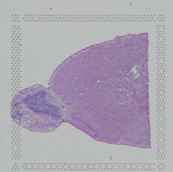
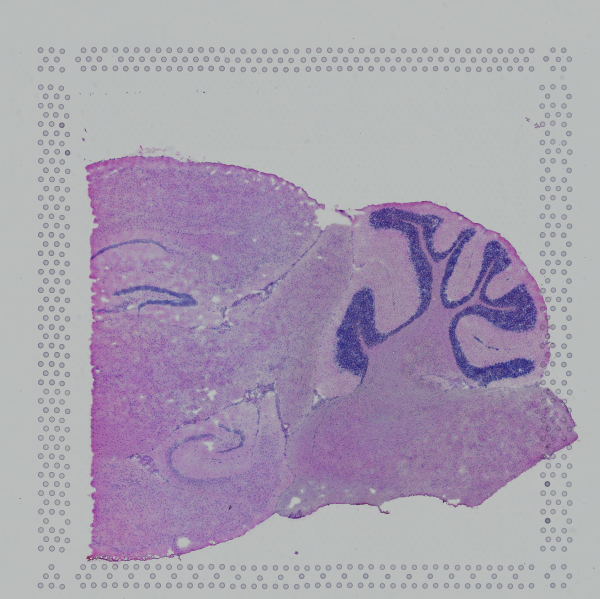
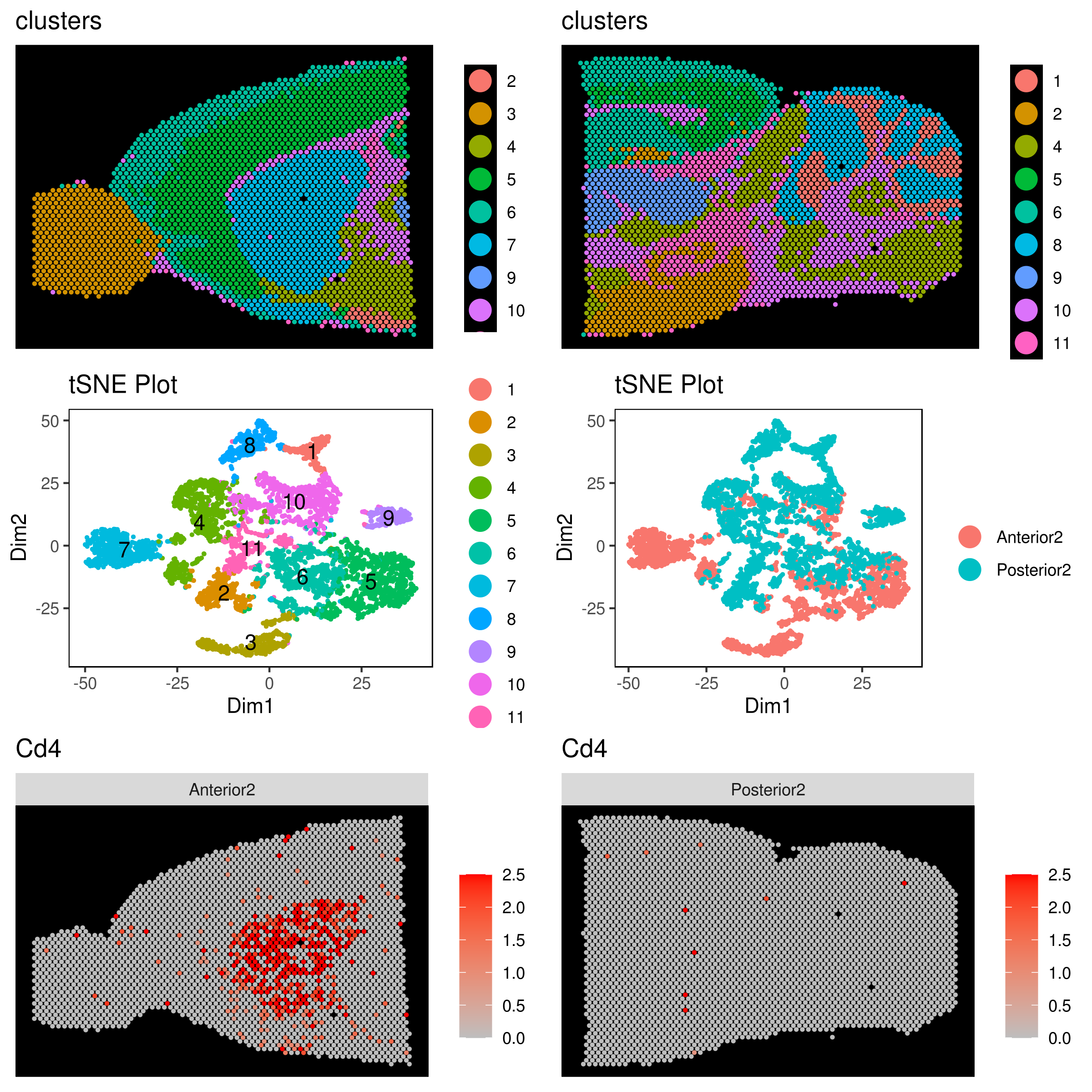
Single cell ATAC sequencing with scRNA-Seq (scATAC-Seq)

library("iCellR") my.data <- load10x("filtered_gene_bc_matrices/")

see the row names

row.names(my.data)

get peak names

ATAC <- grep("^chr",row.names(my.data),value=T)

get scATAC data

MyATAC <- subset(my.data, row.names(my.data) %in% ATAC) head(MyATAC)[1:3]

AAACAGCCAAGTGAAC.1 AAACAGCCACTGACCG.1 AAACAGCCATGATTGT.1

#chr1.181218.181695 0 0 1 #chr1.191296.191699 0 0 0 #chr1.629770.630129 0 0 0 #chr1.633806.634251 0 0 0 #chr1.778422.779040 0 0 0 #chr1.827306.827702 0 0 0

dim(MyATAC)

[1] 21923 6326

get RNA data

MyRNAs <- subset(my.data, !row.names(my.data) %in% ATAC) head(MyRNAs)[1:3]

AAACAGCCAAGTGAAC.1 AAACAGCCACTGACCG.1 AAACAGCCATGATTGT.1

#MIR1302.2HG 0 0 0 #FAM138A 0 0 0 #OR4F5 0 0 0 #AL627309.1 0 0 0 #AL627309.3 0 0 0 #AL627309.2 0 0 0

dim(MyRNAs) #[1] 36633 6326

make iCellR object

my.obj <- make.obj(MyRNAs)

add ATAC-Seq data

my.obj@atac.raw <- MyATAC my.obj@atac.main <- MyATAC

check your object

my.obj

################################### ,--. ,-----. ,--.,--.,------. --'' .--./ ,---. | || || .--. ' ,--.| | | .-. :| || || '--'.' | |' '--'\ --. | || || | --' -----' ----'--'--'`--' '--' ################################### An object of class iCellR version: 1.6.2 Raw/original data dimentions (rows,columns): 24127,6326 Data conditions: no conditions/single sample Row names: MIR1302.2HG,TTLL10.AS1,MRPL20.AS1 ... Columns names: AAACAGCCAAGTGAAC.1,AAACAGCCACTGACCG.1,AAACAGCCATGATTGT.1 ... ################################### QC stats performed:FALSE, PCA performed:FALSE Clustering performed:FALSE, Number of clusters:0 tSNE performed:FALSE, UMAP performed:FALSE, DiffMap performed:FALSE Main data dimensions (rows,columns): 0,0 Normalization factors:,... Imputed data dimensions (rows,columns):0,0 ############## scVDJ-seq ########### VDJ data dimentions (rows,columns):0,0 ############## CITE-seq ############ ADT raw data dimensions (rows,columns):0,0 ADT main data dimensions (rows,columns):0,0 ADT columns names:... ADT row names:... ############## scATAC-seq ############ ATAC raw data dimensions (rows,columns):21923,6326 ATAC main data dimensions (rows,columns):21923,6326 ATAC columns names:AAACAGCCAAGTGAAC.1... ATAC row names:chr1.181218.181695... ############## Spatial ########### Spatial data dimentions (rows,columns):0,0 ########### iCellR object ##########

From here do the regular scRNA-seq as expleind above. See example below

QC

my.obj <- qc.stats(my.obj, s.phase.genes = s.phase, g2m.phase.genes = g2m.phase)

plot as mentioned above

filter

my.obj <- cell.filter(my.obj, min.mito = 0, max.mito = 0.07 , min.genes = 500, max.genes = 4000, min.umis = 0, max.umis = Inf)

normalize RNA

my.obj <- norm.data(my.obj, norm.method = "ranked.glsf", top.rank = 500)

normalize ADT

my.obj <- norm.adt(my.obj)

gene stats

my.obj <- gene.stats(my.obj, which.data = "main.data")

find genes for PCA

my.obj <- make.gene.model(my.obj, my.out.put = "data", dispersion.limit = 1.5, base.mean.rank = 500, no.mito.model = T, mark.mito = T, interactive = F, no.cell.cycle = T, out.name = "gene.model")

run PCA and the rest is as above

my.obj <- run.pca(my.obj, method = "gene.model", gene.list = my.obj@gene.model,data.type = "main")

tSNE

my.obj <- run.pc.tsne(my.obj, dims = 1:10)

UMAP

my.obj <- run.umap(my.obj, dims = 1:10)

KNetL

my.obj <- run.knetl(my.obj, dims = 1:20, zoom = 200, dim.redux = "umap")

clustering based on KNetL

my.obj <- iclust(my.obj, sensitivity = 200, data.type = "knetl")

clustering based on PCA

my.obj <- iclust(my.obj, sensitivity = 100, data.type = "pca", dims=1:10)

check clusters and adjust if needed (optinal)

cluster.plot(my.obj,plot.type = "knetl",interactive = F,cell.size = 0.5,cell.transparency = 1, anno.clust=T)

my.obj <- change.clust(my.obj, change.clust = 3, to.clust = 4)

my.obj <- change.clust(my.obj, change.clust = 3, to.clust = 10)

order clusters

my.obj <- clust.ord(my.obj,top.rank = 500, how.to.order = "distance")

plot

A= cluster.plot(my.obj,plot.type = "pca",interactive = F,cell.size = 0.5,cell.transparency = 1, anno.clust=T) B= cluster.plot(my.obj,plot.type = "umap",interactive = F,cell.size = 0.5,cell.transparency = 1, anno.clust=T) C= cluster.plot(my.obj,plot.type = "tsne",interactive = F,cell.size = 0.5,cell.transparency = 1, anno.clust=T) D= cluster.plot(my.obj,plot.type = "knetl",interactive = F,cell.size = 0.5,cell.transparency = 1, anno.clust=T)

library(gridExtra) png('AllClusts.png', width = 12, height = 10, units = 'in', res = 300) grid.arrange(A,B,C,D) dev.off()

save object

save(my.obj, file = "my.obj.Robj")

find markers

marker.genes <- findMarkers(my.obj, data.type = "main", fold.change = 2, padjval = 0.1, uniq = F, positive = T)

marker.genes1 <- cbind(row = rownames(marker.genes), marker.genes) write.table((marker.genes1),file="marker.genes.tsv", sep="\t", row.names =F)

MyGenes <- top.markers(marker.genes, topde = 10, min.base.mean = 0.2, filt.ambig = F) MyGenes <- unique(MyGenes)

png('heatmap_gg_genes.png', width = 10, height = 10, units = 'in', res = 300) heatmap.gg.plot(my.obj, gene = MyGenes, interactive = F, cluster.by = "clusters",cell.sort = F, conds.to.plot = NULL) dev.off()

Work on scATAC data (normalize and find marker peaks for each cluster)

normalize ACAT

my.obj <- norm.data(my.obj, norm.method = "ranked.glsf", top.rank = 500, ATAC.data = TRUE, ATAC.filter = TRUE)

marker.peaks <- findMarkers(my.obj, data.type = "atac", fold.change = 2, padjval = 0.1, uniq = F, positive = T)

marker.peaks1 <- cbind(row = rownames(marker.peaks), marker.peaks) write.table((marker.peaks1),file="marker.peaks.tsv", sep="\t", row.names =F)

head(marker.peaks1)

row baseMean baseSD

#chr17.64986035.64986113 chr17.64986035.64986113 0.01217359 0.18257818 #chr1.26542287.26542678 chr1.26542287.26542678 0.05828764 0.80077656 #chr4.8199063.8199275 chr4.8199063.8199275 0.04280424 0.56205649 #chr20.50274929.50275237 chr20.50274929.50275237 0.04684509 0.63361490 #chr2.218382038.218382236 chr2.218382038.218382236 0.03122394 0.31153105 #chr11.1760469.1760814 chr11.1760469.1760814 0.07050175 0.63322284

AvExpInCluster AvExpInOtherClusters foldChange

#chr17.64986035.64986113 0.07868394 0.002346603 33.530999 #chr1.26542287.26542678 0.33849093 0.016887273 20.044144 #chr4.8199063.8199275 0.24803497 0.012481148 19.872769 #chr20.50274929.50275237 0.27007513 0.013862584 19.482308 #chr2.218382038.218382236 0.17736269 0.009631770 18.414340 #chr11.1760469.1760814 0.39043782 0.023230813 16.806894

log2FoldChange pval padj clusters

#chr17.64986035.64986113 5.067424 1.187697e-05 2.875415e-02 1 #chr1.26542287.26542678 4.325109 3.653916e-05 8.539202e-02 1 #chr4.8199063.8199275 4.312721 6.059691e-06 1.489472e-02 1 #chr20.50274929.50275237 4.284093 2.871301e-05 6.779143e-02 1 #chr2.218382038.218382236 4.202758 6.359572e-10 1.677019e-06 1 #chr11.1760469.1760814 4.070981 6.813447e-11 1.800794e-07 1

gene cluster_1 cluster_2

#chr17.64986035.64986113 chr17.64986035.64986113 0.0786839378 0.000000000 #chr1.26542287.26542678 chr1.26542287.26542678 0.3384909326 0.008895062 #chr4.8199063.8199275 chr4.8199063.8199275 0.2480349741 0.038672840 #chr20.50274929.50275237 chr20.50274929.50275237 0.2700751295 0.028703704 #chr2.218382038.218382236 chr2.218382038.218382236 0.1773626943 0.000000000 #chr11.1760469.1760814 chr11.1760469.1760814 0.3904378238 0.004537037

cluster_3 cluster_4 cluster_5 cluster_6

#chr17.64986035.64986113 0.000000000 0.0000000000 0.0006934750 0.0010038760 #chr1.26542287.26542678 0.031485714 0.0029244992 0.0052261002 0.0041264535 #chr4.8199063.8199275 0.000000000 0.0007226502 0.0027450683 0.0113212209 #chr20.50274929.50275237 0.027092857 0.0121741140 0.0041820941 0.0051516473 #chr2.218382038.218382236 0.004292857 0.0042095532 0.0006722307 0.0038561047 #chr11.1760469.1760814 0.071678571 0.0177288136 0.0141820941 0.0061099806

cluster_7 cluster_8

#chr17.64986035.64986113 0.003099029 0.009080357 #chr1.26542287.26542678 0.047110680 0.044484375 #chr4.8199063.8199275 0.014819417 0.028651786 #chr20.50274929.50275237 0.025499029 0.028765625 #chr2.218382038.218382236 0.011988350 0.035508929 #chr11.1760469.1760814 0.042093204 0.050708705

MyGenes <- top.markers(marker.peaks, topde = 10, min.base.mean = 0.2, filt.ambig = F) MyGenes <- unique(MyGenes)

png('heatmap_gg_peaks.png', width = 10, height = 10, units = 'in', res = 300) heatmap.gg.plot(my.obj, gene = MyGenes, interactive = F, cluster.by = "clusters",cell.sort = F, conds.to.plot = NULL, data.type = "atac") dev.off()

my.obj <- run.impute(my.obj,data.type = "knetl", nn = 10, ATAC.data = FALSE)

you can also find avarage peak intensity per cluster

my.obj <- clust.avg.exp(my.obj, data.type = "atac") head(my.obj@clust.avg)

#gene cluster_1 cluster_2 ... #chr1.100037799.100038931 0.38238731 0.36750000 ... #chr1.100132733.100133298 0.11195725 1.13593827 ... #chr1.100249637.100250160 0.09851425 0.09511728 ... #chr1.100265992.100266479 0.06768394 0.17707407 ... #chr1.10032488.10033387 0.35273705 0.14885802 ... #chr1.100352150.100352921 0.12006088 0.00000000 ...

find out which cluster has the highest number

dat <- as.data.frame(t((my.obj@clust.avg)[,-1])) dat <- hto.anno(hto.data = dat)

head(dat$assignment.annotatio) #[1] cluster_1 cluster_2 cluster_4 cluster_2 cluster_3 cluster_4 #8 Levels: cluster_1 cluster_2 cluster_3 cluster_4 cluster_5 ... cluster_8

Peak analysis

make a bed file per cluster from the marker.peaks file you made up here

make.bed(marker.peaks)

load packages

library(ChIPseeker) library(clusterProfiler)

load genome

require(TxDb.Hsapiens.UCSC.hg38.knownGene) txdb <- TxDb.Hsapiens.UCSC.hg38.knownGene Anno="org.Hs.eg.db"

load bed files

Mylist1 = list.files(pattern=".bed") Mylist1

Mylist <- as.list(Mylist1) NAMES <- gsub('_peaks.bed','',Mylist1) names(Mylist) <- NAMES files <- Mylist files

perform analysis (example)

promoter <- getPromoters(TxDb=txdb, upstream=3000, downstream=3000) tagMatrixList <- lapply(files, getTagMatrix, windows=promoter)

pdf("Plot_ProfileLineAll.pdf") plotAvgProf(tagMatrixList, xlim=c(-3000, 3000)) dev.off()

pdf('Plot_ProfileLine.pdf', width = 8, height = 10) plotAvgProf(tagMatrixList, xlim=c(-3000, 3000), facet="row") dev.off()

pdf("Plot_heatmaps.pdf", width = 50, height = 6) tagHeatmap(tagMatrixList, xlim=c(-3000, 3000), color=NULL) dev.off()

annotate

peakAnnoList <- lapply(files, annotatePeak, TxDb=txdb, tssRegion=c(-3000, 3000), verbose=FALSE)

plot annotatin

pdf("Plot_AnnoBar.pdf") plotAnnoBar(peakAnnoList) dev.off()

############### peak annotation

peakAnnoList <- lapply(files, annotatePeak, TxDb=txdb, tssRegion=c(-3000, 3000), verbose=FALSE, annoDb=Anno)

capture.output(peakAnnoList, file = "peakAnnoList.txt")

genes = lapply(peakAnnoList, function(i) as.data.frame(i))

lapply(1:length(genes), function(i) write.table(genes[[i]], file = paste0(names(genes[i]), ".xls"), row.names = FALSE, sep="\t"))

Merging scATAC files with different intervals (as dipicted in bedtools website)

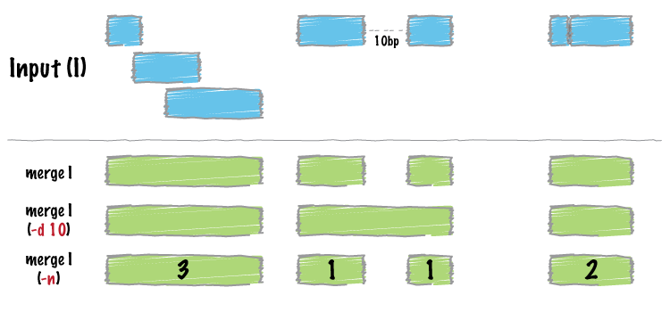
# Let's say you have 2 files that you need to merege

# example file
C <- load10x("count-JJsn_C_cDNA/",gene.name = 2)
M <- load10x("count-JJsn_M_cDNA/",gene.name = 2)

ATAC.C <- grep("^chr",row.names(C),value=T)
ATAC.M <- grep("^chr",row.names(M),value=T)

MyATAC.C <- subset(C, row.names(C) %in% ATAC.C)
MyATAC.M <- subset(M, row.names(M) %in% ATAC.M)

head(MyATAC.C)[1:3]

C <- MyATAC.C
M <- MyATAC.M

dim(C)
#[1] 58678  4211
dim(M)
#[1] 57776  4736

f1 <- row.names(C)
f2 <- row.names(M)

all.peaks <- c(f1,f2)
length(all.peaks)
#[1] 116454

# make a bed file
chr <- as.character(as.matrix(data.frame(do.call('rbind', strsplit(as.character(all.peaks),'.',fixed=TRUE)))[1]))
start <- data.frame(do.call('rbind', strsplit(as.character(all.peaks),'.',fixed=TRUE)))[2]
end <- data.frame(do.call('rbind', strsplit(as.character(all.peaks),'.',fixed=TRUE)))[3]

DAT <- as.data.frame(chr)
DAT$start <- as.numeric(as.matrix(start))
DAT$end <- as.numeric(as.matrix(end))
head(DAT)
#   chr  start    end
#1 chr1 181218 181695
#2 chr1 191296 191699
#3 chr1 629770 630129
#4 chr1 633806 634251
#5 chr1 778422 779040
#6 chr1 827306 827702

# make Genomic Ranges
library("GenomicRanges")

all.gr <- GRanges(seqnames=DAT$chr,ranges=IRanges(start=DAT$start,end=DAT$end))

all.gr
#GRanges object with ?? ranges and 0 metadata columns:
#       seqnames          ranges strand
#          <Rle>       <IRanges>  <Rle>
#   [1]     chr1   181218-181695      *
#   [2]     chr1   191296-191699      *
#   [3]     chr1   629770-630129      *
#   [4]     chr1   633806-634251      *
#   [5]     chr1   778422-779040      *
#   ...      ...             ...    ...
#  [52]     chr1 1303892-1306216      *
#  [53]     chr1 1307242-1309359      *
#  [54]     chr1 1324425-1325236      *
#  [55]     chr1 1348940-1349958      *
#  [56]     chr1 1372031-1372220      *
#  -------
#  seqinfo: 1 sequence from an unspecified genome; no seqlengths

################## sort and merge the peaks

mrg <- reduce(all.gr)

#Before merge
length(all.gr)
#[1] 116454
#after merge
length(mrg)
#[1] 71426

########################## choose file and give name
MyFile <- f1
name="f1_new.bed"
########################## copy paste the code here to make a new bed file
########################## the new bed has the old and new intervals (new intervals to be replaced with old)

chr <- as.character(as.matrix(data.frame(do.call('rbind', strsplit(as.character(MyFile),'.',fixed=TRUE)))[1]))
start <- data.frame(do.call('rbind', strsplit(as.character(MyFile),'.',fixed=TRUE)))[2]
end <- data.frame(do.call('rbind', strsplit(as.character(MyFile),'.',fixed=TRUE)))[3]
# make a bed file
DAT <- as.data.frame(chr)
DAT$start <- as.numeric(as.matrix(start))
DAT$end <- as.numeric(as.matrix(end))
MyFile <- DAT

# make intrval file to replace to new regions
MyFile.gr <- GRanges(seqnames=MyFile$chr,ranges=IRanges(start=MyFile$start,end=MyFile$end))

OverLap <- findOverlaps(MyFile.gr, mrg)

OLD1 <- (OverLap@from)
NEW1 <- (OverLap@to)

OLD = MyFile.gr[OLD1]
NEW = mrg[NEW1]

chr <- as.character(OLD@seqnames)
DAT <- as.data.frame(chr)
DAT$start <- OLD@ranges@start
DAT$end <- (OLD@ranges@start + OLD@ranges@width) - 1

DAT$new.chr<- as.character(NEW@seqnames)
DAT$new.start <- NEW@ranges@start
DAT$new.end <- (NEW@ranges@start + NEW@ranges@width) - 1

head(DAT)
#   chr   start     end new.chr new.start new.end
#1 chr1 3247563 3248453    chr1   3247563 3248453
#2 chr1 3360706 3361554    chr1   3360706 3361554
#3 chr1 3552372 3553230    chr1   3552372 3553230
#4 chr1 3645171 3646034    chr1   3645093 3646034
#5 chr1 3670318 3671081    chr1   3670318 3671090
#6 chr1 3671326 3672230    chr1   3671314 3672230

dim(DAT)
#58678     6
length(MyFile.gr)
#58678

# diff

have = mrg[unique(NEW1)]
dontHave = mrg[-unique(NEW1)]

ADD <- dontHave
L <- length(as.character(ADD@seqnames))
chr <-rep("NA",L)
DAT1 <- as.data.frame(chr)
DAT1$start <- rep("NA",L)
DAT1$end <- rep("NA",L)
DAT1$new.chr<- as.character(ADD@seqnames)
DAT1$new.start <- ADD@ranges@start
DAT1$new.end <- (ADD@ranges@start + ADD@ranges@width) - 1

Final.DAT <- rbind(DAT,DAT1)

##### Write

write.table(Final.DAT,name,row.names=FALSE,sep="\t", quote = FALSE)

### reapeat this process for f2 (M) as well

# The first 3 columns are the original peaks and the last 3 are the ones that need to be replaced with original one. The NA peaks would also get the new peak ids but in the matrix the cells will have 0 for expressions. To do this use the iCellR function replace.peak.id.

MyATAC.C <- replace.peak.id(atac.data=MyATAC.C, bed.file = Final.DAT.C)
MyATAC.M <- replace.peak.id(atac.data=MyATAC.M, bed.file = Final.DAT.M)

# finally aggregate the samples and add to iCellR object

my.atac.data <- data.aggregation(samples = c("MyATAC1","MyATAC2","MyATAC3"),
    condition.names = c("WT","KO","Ctrl"))
    
# add ATAC-Seq data
my.obj@atac.raw <- my.atac.data
my.obj@atac.main <- my.atac.data