StabMap: Stabilised mosaic single cell data integration using unshared features (original) (raw)
Introduction
StabMap is a technique for performing mosaic single cell data integration.
In this vignette we will elaborate on how these steps are implemented in the StabMap package.
Load data
mae <- scMultiome("pbmc_10x", mode = "*", dry.run = FALSE, format = "MTX")Perform some exploration of this data.
## A MultiAssayExperiment object of 2 listed
##  experiments with user-defined names and respective classes.
##  Containing an ExperimentList class object of length 2:
##  [1] atac: SingleCellExperiment with 108344 rows and 10032 columns
##  [2] rna: SingleCellExperiment with 36549 rows and 10032 columns
## Functionality:
##  experiments() - obtain the ExperimentList instance
##  colData() - the primary/phenotype DataFrame
##  sampleMap() - the sample coordination DataFrame
##  `$`, `[`, `[[` - extract colData columns, subset, or experiment
##  *Format() - convert into a long or wide DataFrame
##  assays() - convert ExperimentList to a SimpleList of matrices
##  exportClass() - save data to flat files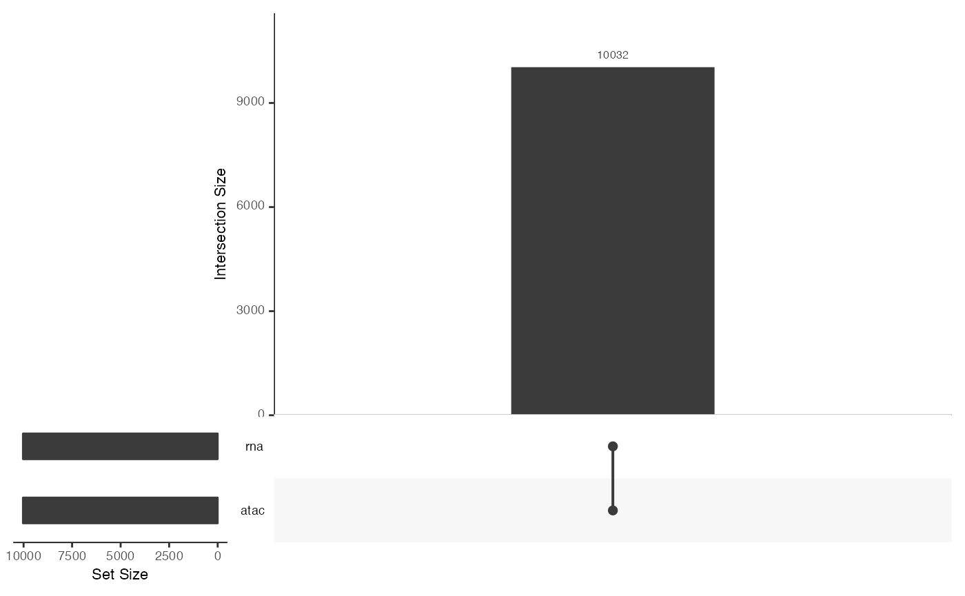
## DataFrame with 6 rows and 6 columns
##                  nCount_RNA nFeature_RNA nCount_ATAC nFeature_ATAC
##                   <integer>    <integer>   <integer>     <integer>
## AAACAGCCAAGGAATC       8380         3308       55582         13878
## AAACAGCCAATCCCTT       3771         1896       20495          7253
## AAACAGCCAATGCGCT       6876         2904       16674          6528
## AAACAGCCAGTAGGTG       7614         3061       39454         11633
## AAACAGCCAGTTTACG       3633         1691       20523          7245
## AAACAGCCATCCAGGT       7782         3028       22412          8602
##                                celltype broad_celltype
##                             <character>    <character>
## AAACAGCCAAGGAATC      naive CD4 T cells       Lymphoid
## AAACAGCCAATCCCTT     memory CD4 T cells       Lymphoid
## AAACAGCCAATGCGCT      naive CD4 T cells       Lymphoid
## AAACAGCCAGTAGGTG      naive CD4 T cells       Lymphoid
## AAACAGCCAGTTTACG     memory CD4 T cells       Lymphoid
## AAACAGCCATCCAGGT non-classical monocy..        Myeloid
## [1] 36549 10032## [1] "atac" "rna"Normalise and select features for the RNA modality.
## [1] 952sce.rna <- sce.rna[hvgs,]Normalise and select features for the ATAC modality.
## [1] 108344 10032sce.atac <- experiments(mae)[["atac"]]
# Normalise
sce.atac <- logNormCounts(sce.atac)
# Feature selection using highly variable peaks
# And adding matching peaks to genes
decomp <- modelGeneVar(sce.atac)
hvgs <- rownames(decomp)[decomp$mean>0.25
& decomp$p.value <= 0.05]
length(hvgs)## [1] 788sce.atac <- sce.atac[hvgs,]Create a composite full data matrix by concatenating.
## [1] 1740 10032## assayType
## atac rna
## 788 952We will simulate a situation where half of the cells correspond to the Multiome modality, and half of the cells correspond to the RNA modality. Our goal is to then generate a joint embedding of the cells using all data, and to impute the missing ATAC values from the RNA modality cells.
## dataType
## Multiome      RNA
##     4983     5049
assay_list = list(
RNA = logcounts_all[assayType %in% c("rna"), dataType %in% c("RNA")],
Multiome = logcounts_all[assayType %in% c("rna", "atac"), dataType %in% c("Multiome")]
)
lapply(assay_list, dim)## $RNA
## [1] 952 5049
##
## $Multiome
## [1] 1740 4983## $RNA
## [1] "dgCMatrix"
## attr(,"package")
## [1] "Matrix"
##
## $Multiome
## [1] "dgCMatrix"
## attr(,"package")
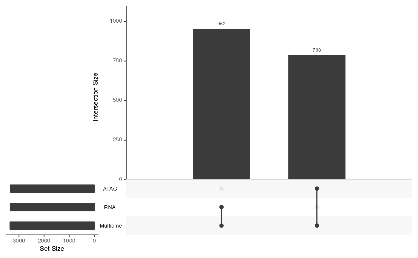
## [1] "Matrix"Examine the shared features between the two datasets using[mosaicDataUpSet()](../reference/mosaicDataUpSet.html).
## Loading required package: UpSetR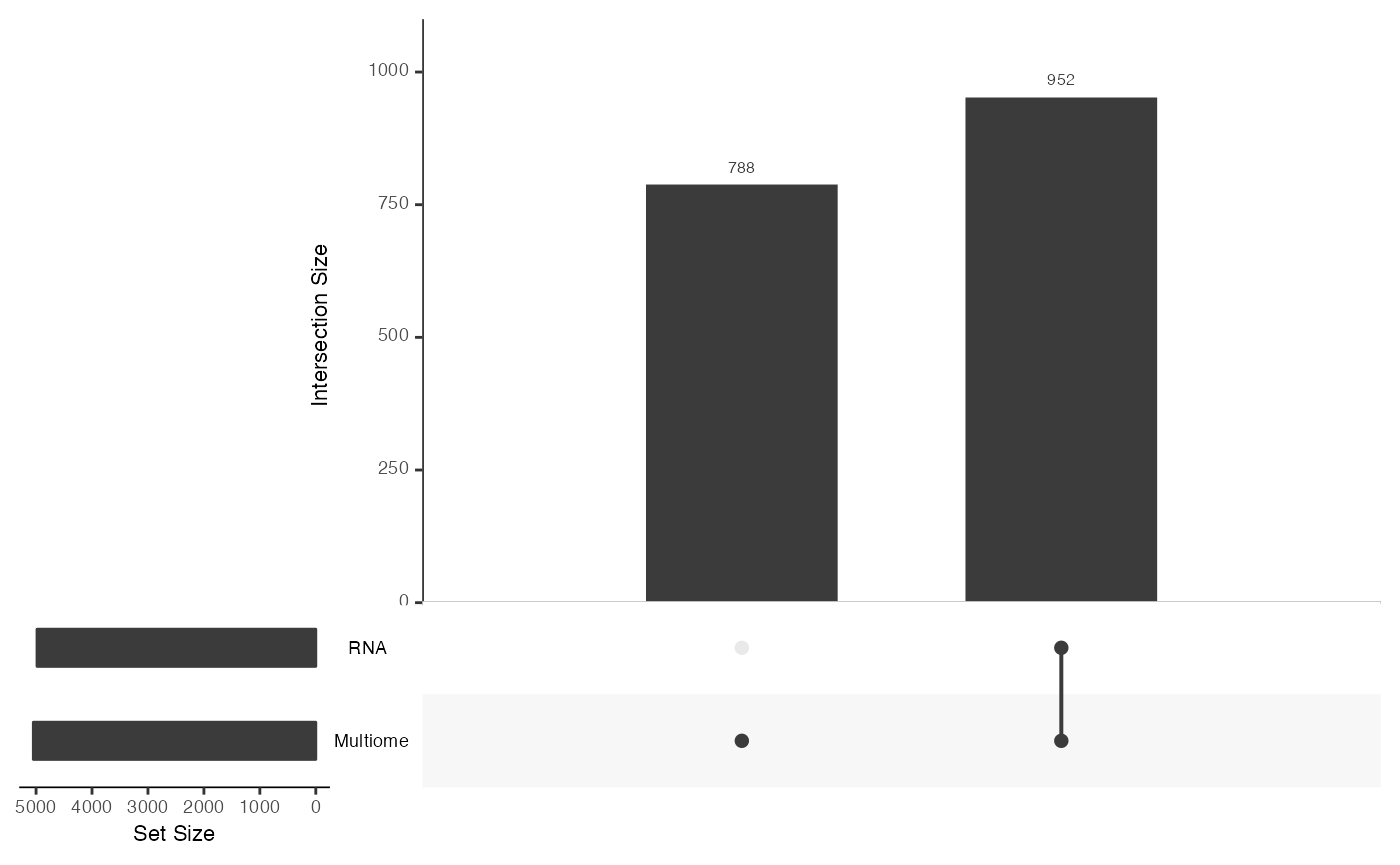
From this we note that there are shared features between the RNA and Multiome datasets, but there are many features that are observed only in the Multiome dataset and not the RNA - as we had constructed.
We can understand the [mosaicDataTopology()](../reference/mosaicDataTopology.html) of these datasets, which generates an igraph object, which can be inspected and plotted.
## IGRAPH 073624a UN-- 2 1 --
## + attr: name (v/c), frame.color (v/c), color (v/c), label.color (v/c),
## | label.family (v/c)
## + edge from 073624a (vertex names):
## [1] RNA--Multiome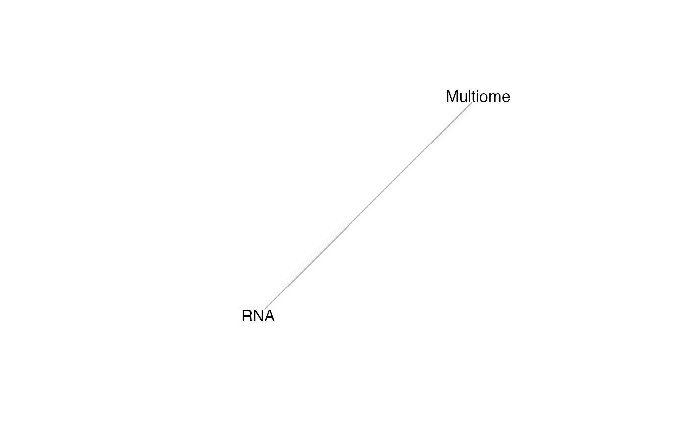
From this we note that the datasets RNA and Multiome share at least some features. StabMap requires that the mosaic data topology network be connected, that is, that there should be a path between every pair of nodes in the network.
We generate a common joint embedding for these data using StabMap. Since the Multiome data contains all features, we treat this as the reference dataset. Since we already examined the mosaic data topology, we set plot = FALSE.
stab = stabMap(assay_list,
               reference_list = c("Multiome"),
               plot = FALSE)
## Loading required package: scater## Loading required package: ggplot2## treating "Multiome" as reference## generating embedding for path with reference "Multiome": "Multiome"## generating embedding for path with reference "Multiome": "RNA" -> "Multiome"## [1] 10032 50## Multiome_PC1 Multiome_PC2 Multiome_PC3 Multiome_PC4
## AAACAGCCAAGGAATC 7.914327 -1.3703933 2.8728293 0.2016397
## AAACAGCCAGTAGGTG 9.607305 -2.7416853 2.4949054 -0.1657897
## AAACATGCACCGGCTA 3.551898 -1.3632683 -9.1696271 0.3137612
## AAACATGCAGGGAGCT 4.298441 -1.1046894 -11.2718261 1.2654560
## AAACCGAAGCTGGACC -9.870562 -0.6587611 0.3410302 0.3198895
## Multiome_PC5
## AAACAGCCAAGGAATC 0.9913363
## AAACAGCCAGTAGGTG 1.5115966
## AAACATGCACCGGCTA 1.6221187
## AAACATGCAGGGAGCT 3.1555720
## AAACCGAAGCTGGACC 4.0684566We can reduce the dimension further using non-linear approaches such as UMAP.
stab_umap = calculateUMAP(t(stab))
dim(stab_umap)
## [1] 10032 2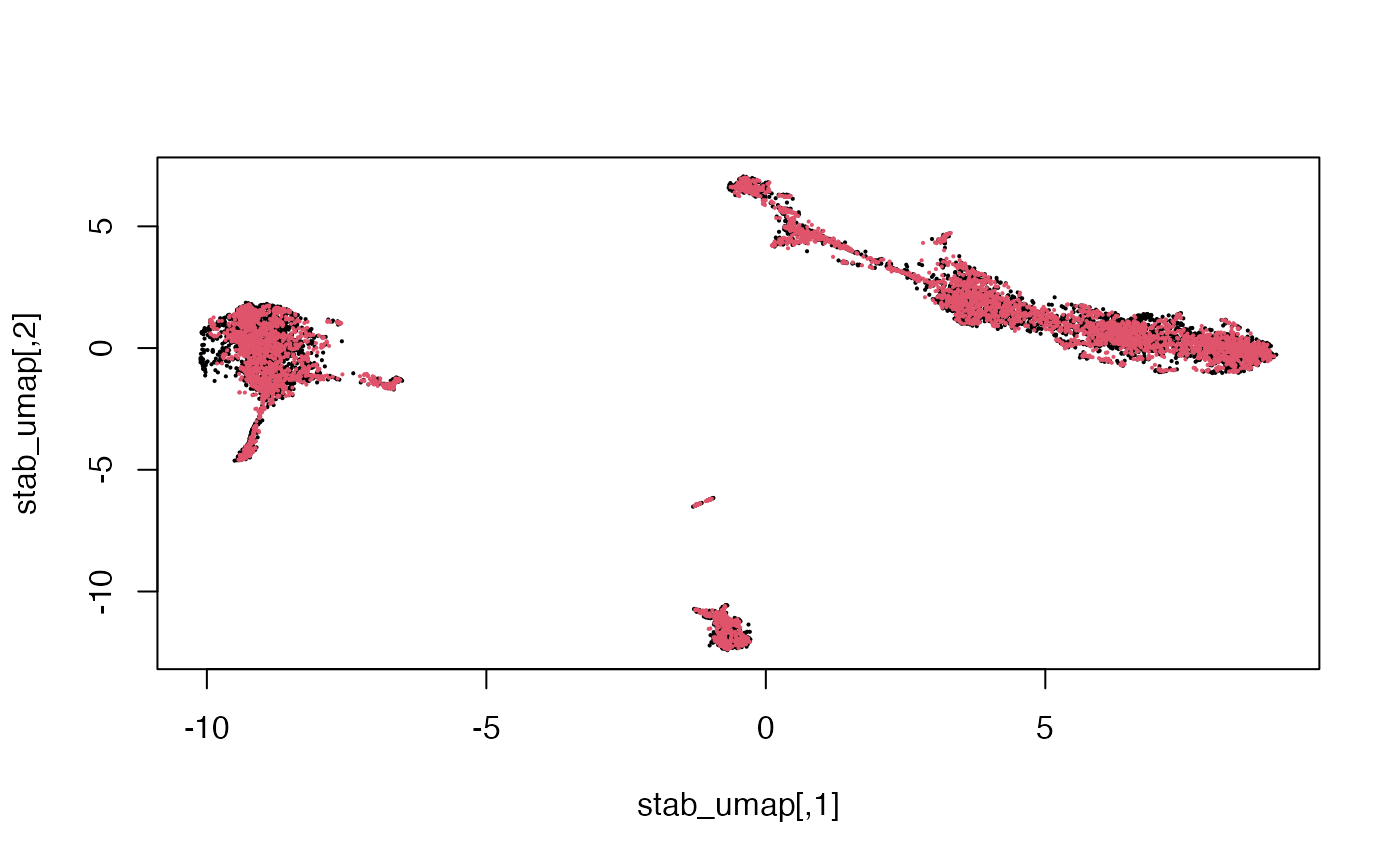
Here we see that the RNA and Multiome cells are fairly well-mixed.
Data imputation after StabMap
Given the joint embedding, we can predict the missing ATAC values using [imputeEmbedding()](../reference/imputeEmbedding.html). We provide the data list, the joint embedding as output from [stabMap()](../reference/StabMap.html). We set the Multiome cells as reference and the RNA cells as query. This is useful for downstream visualisation or further interpretation.
## Loading required package: BiocNeighbors## Loading required package: slam## Loading required package: Matrix##
## Attaching package: 'Matrix'## The following object is masked from 'package:S4Vectors':
##
## expand## [1] "list"## [1] "Multiome"## $Multiome
## [1] 1740 5049imp[["Multiome"]][1:5,1:5]## 5 x 5 sparse Matrix of class "dgCMatrix"
## AAACAGCCAATCCCTT AAACAGCCAATGCGCT AAACAGCCAGTTTACG AAACAGCCATCCAGGT
## CA6 . . . .
## CNR2 . . . .
## IFNLR1 . . . .
## RCAN3 1.387121 1.787342 1.520869 .
## ZNF683 . . . .
## AAACATGCAAGGTCCT
## CA6 1.177289
## CNR2 .
## IFNLR1 .
## RCAN3 1.101005
## ZNF683 .Indirect mosaic data integration with StabMap
StabMap is a flexible framework for mosaic data integration, and can still integrate data even when there are pairs of datasets that share no features at all. So long as there is a path connecting the datasets along the mosaic data topology (and the underlying assumption that the shared features along these paths contain information), then we can extract meaningful joint embeddings. To demonstrate this, we will simulate three data sources.
dataTypeIndirect = setNames(sample(c("RNA", "Multiome", "ATAC"), ncol(logcounts_all),
                                   prob = c(0.3,0.3, 0.3), replace = TRUE),
                            colnames(logcounts_all))
table(dataTypeIndirect)
## dataTypeIndirect
## ATAC Multiome RNA
## 3338 3359 3335assay_list_indirect = list(
RNA = logcounts_all[assayType %in% c("rna"), dataTypeIndirect %in% c("RNA")],
Multiome = logcounts_all[assayType %in% c("rna", "atac"), dataTypeIndirect %in% c("Multiome")],
ATAC = logcounts_all[assayType %in% c("atac"), dataTypeIndirect %in% c("ATAC")]
)
lapply(assay_list_indirect, dim)## $RNA
## [1] 952 3335
##
## $Multiome
## [1] 1740 3359
##
## $ATAC
## [1] 788 3338lapply(assay_list_indirect, class)## $RNA
## [1] "dgCMatrix"
## attr(,"package")
## [1] "Matrix"
##
## $Multiome
## [1] "dgCMatrix"
## attr(,"package")
## [1] "Matrix"
##
## $ATAC
## [1] "dgCMatrix"
## attr(,"package")
## [1] "Matrix"Using [mosaicDataUpSet()](../reference/mosaicDataUpSet.html), we note that there are no shared features between the ATAC and RNA datasets. We might be able to match features by extracting genomic positions and making the “central dogma assumption”, that is, that the peaks associated with a genomic position overlapping a gene should correspond to positive gene expression for that gene. However, we need not make this assumption for the data integration to be performed.
We can understand the [mosaicDataTopology()](../reference/mosaicDataTopology.html) of these datasets, which generates an igraph object, which can be inspected and plotted.
## IGRAPH 4f4fa5d UN-- 3 2 --
## + attr: name (v/c), frame.color (v/c), color (v/c), label.color (v/c),
## | label.family (v/c)
## + edges from 4f4fa5d (vertex names):
## [1] RNA     --Multiome Multiome--ATAC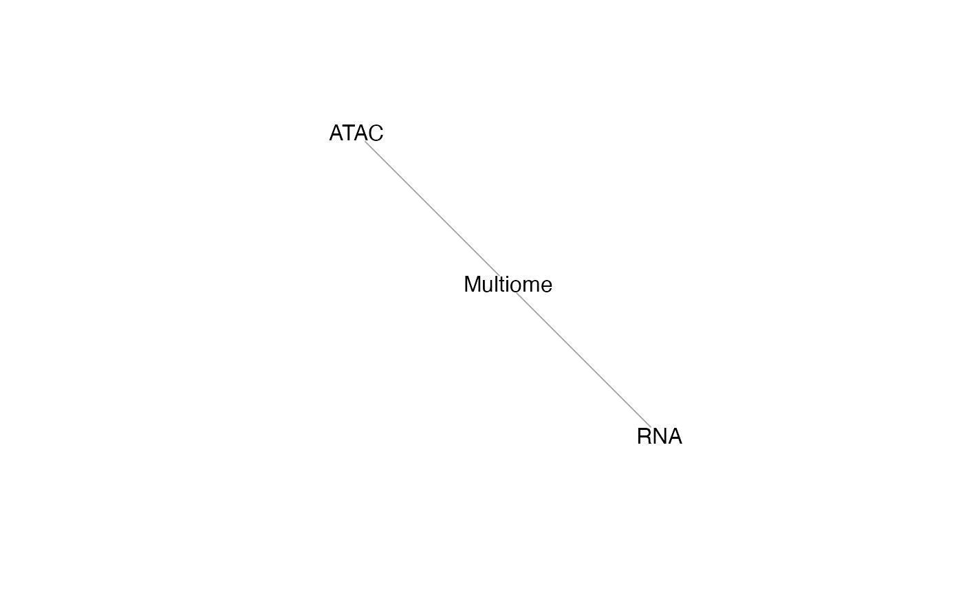
StabMap only requires that the mosaic data topology network be connected, that is, that there should be a path between every pair of nodes in the network. Since there is a path between RNA and ATAC (via Multiome), we can proceed.
We now generate a common joint embedding for these data using StabMap. Since the Multiome data contains all features, we again treat this as the reference dataset. Since we already examined the mosaic data topology, we set plot = FALSE.
stab_indirect = stabMap(assay_list_indirect,
                        reference_list = c("Multiome"),
                        plot = FALSE)
## treating "Multiome" as reference## generating embedding for path with reference "Multiome": "Multiome"## generating embedding for path with reference "Multiome": "RNA" -> "Multiome"## generating embedding for path with reference "Multiome": "ATAC" -> "Multiome"## [1] 10032 50## Multiome_PC1 Multiome_PC2 Multiome_PC3 Multiome_PC4
## AAACAGCCAATCCCTT 6.859810 -1.540596 -1.843308 -0.16435493
## AAACATGCAGCAAGTG 5.570928 -2.379867 2.911351 2.32630567
## AAACATGCAGGGAGCT 4.550189 -1.769688 -13.014403 -0.30613633
## AAACCAACACTAAGAA 7.888117 -1.354557 3.365346 -0.09086506
## AAACCAACAGGATGGC 6.426812 -1.347158 1.944541 -0.12714915
## Multiome_PC5
## AAACAGCCAATCCCTT -1.5442658
## AAACATGCAGCAAGTG -1.7983382
## AAACATGCAGGGAGCT 1.9258897
## AAACCAACACTAAGAA 0.6042899
## AAACCAACAGGATGGC -1.8859162We can reduce the dimension further using non-linear approaches such as UMAP.
stab_indirect_umap = calculateUMAP(t(stab_indirect))
dim(stab_indirect_umap)
## [1] 10032 2plot(stab_indirect_umap, pch = 16, cex = 0.3,
col = factor(dataTypeIndirect[rownames(stab_indirect)]))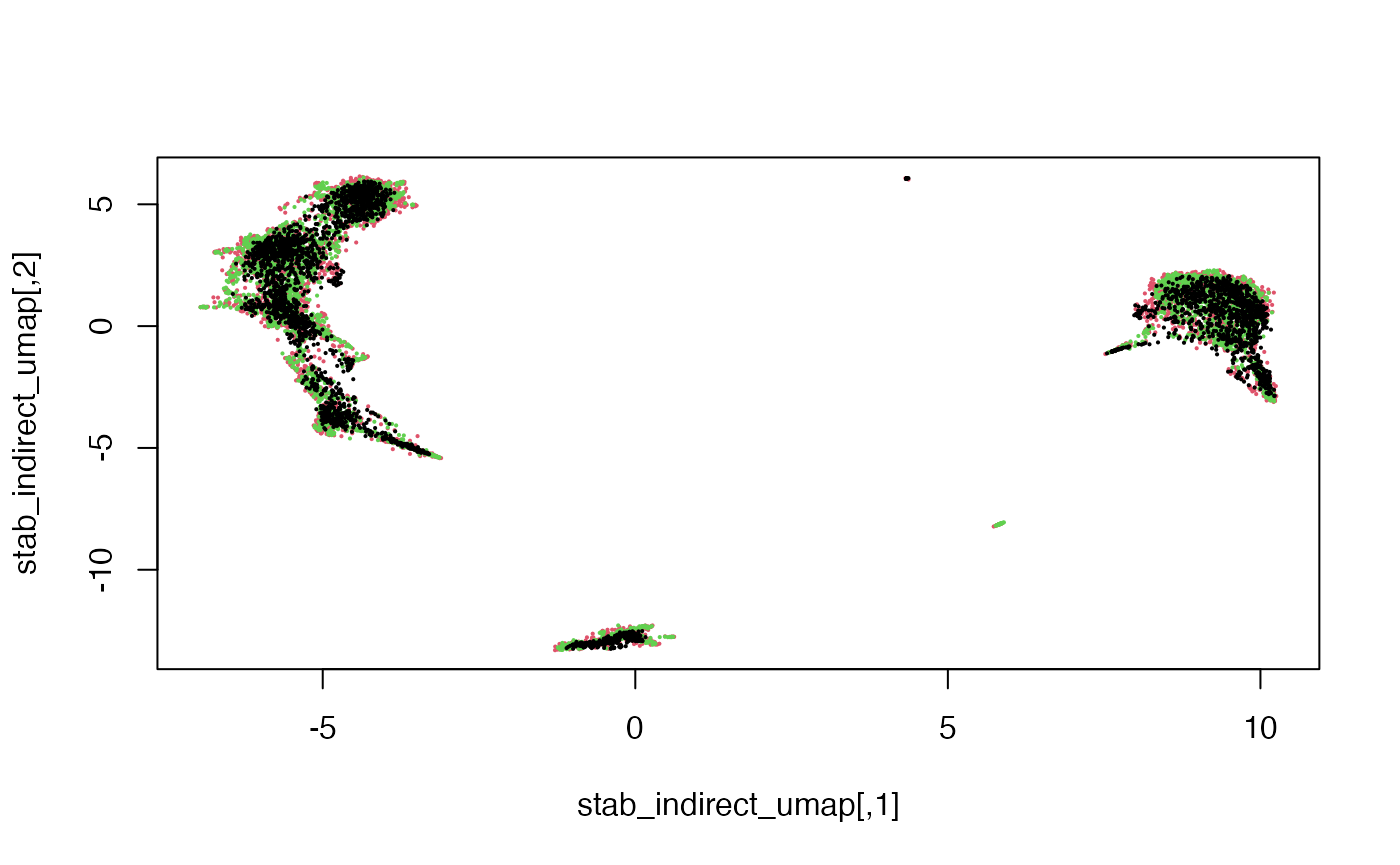
Here we see that the RNA, ATAC and Multiome cells are fairly well-mixed.
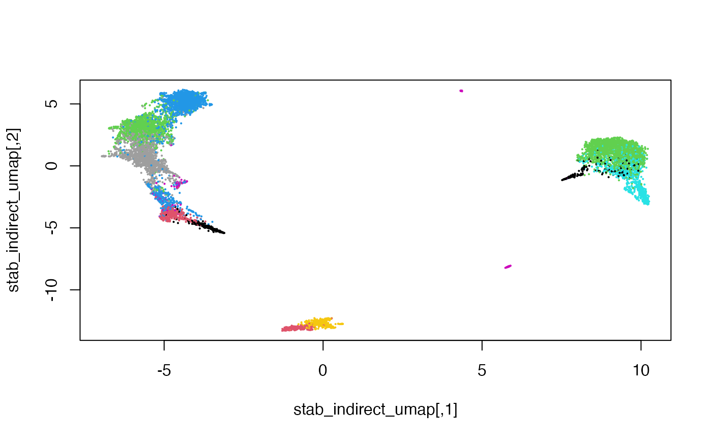
Colouring the cells by their original cell type, we can also see that the mosaic data integration is meaningful.
Session Info
## R version 4.2.1 (2022-06-23)
## Platform: x86_64-apple-darwin17.0 (64-bit)
## Running under: macOS Catalina 10.15.7
##
## Matrix products: default
## BLAS:   /Library/Frameworks/R.framework/Versions/4.2/Resources/lib/libRblas.0.dylib
## LAPACK: /Library/Frameworks/R.framework/Versions/4.2/Resources/lib/libRlapack.dylib
##
## locale:
## [1] en_GB.UTF-8/en_GB.UTF-8/en_GB.UTF-8/C/en_GB.UTF-8/en_GB.UTF-8
##
## attached base packages:
## [1] stats4    stats     graphics  grDevices utils     datasets  methods
## [8] base
##
## other attached packages:
##  [1] Matrix_1.5-1                slam_0.1-50
##  [3] BiocNeighbors_1.14.0        scater_1.24.0
##  [5] ggplot2_3.3.6               UpSetR_1.4.0
##  [7] scran_1.24.0                scuttle_1.6.2
##  [9] SingleCellExperiment_1.18.0 SingleCellMultiModal_1.8.0
## [11] MultiAssayExperiment_1.22.0 SummarizedExperiment_1.26.1
## [13] Biobase_2.56.0              GenomicRanges_1.48.0
## [15] GenomeInfoDb_1.32.2         IRanges_2.30.0
## [17] S4Vectors_0.34.0            BiocGenerics_0.42.0
## [19] MatrixGenerics_1.8.1        matrixStats_0.62.0
## [21] StabMap_0.1.8               igraph_1.3.4
## [23] BiocStyle_2.24.0
##
## loaded via a namespace (and not attached):
##   [1] AnnotationHub_3.4.0           BiocFileCache_2.4.0
##   [3] systemfonts_1.0.4             plyr_1.8.7
##   [5] BiocParallel_1.30.3           digest_0.6.29
##   [7] htmltools_0.5.3               viridis_0.6.2
##   [9] magick_2.7.3                  fansi_1.0.3
##  [11] magrittr_2.0.3                memoise_2.0.1
##  [13] ScaledMatrix_1.4.0            SpatialExperiment_1.6.0
##  [15] cluster_2.1.3                 limma_3.52.2
##  [17] Biostrings_2.64.0             R.utils_2.12.0
##  [19] pkgdown_2.0.6                 colorspace_2.0-3
##  [21] ggrepel_0.9.1                 blob_1.2.3
##  [23] rappdirs_0.3.3                textshaping_0.3.6
##  [25] xfun_0.31                     dplyr_1.0.9
##  [27] crayon_1.5.1                  RCurl_1.98-1.8
##  [29] jsonlite_1.8.0                glue_1.6.2
##  [31] gtable_0.3.0                  zlibbioc_1.42.0
##  [33] XVector_0.36.0                DelayedArray_0.22.0
##  [35] BiocSingular_1.12.0           DropletUtils_1.16.0
##  [37] Rhdf5lib_1.18.2               HDF5Array_1.24.2
##  [39] abind_1.4-5                   scales_1.2.0
##  [41] DBI_1.1.3                     edgeR_3.38.4
##  [43] Rcpp_1.0.9                    viridisLite_0.4.0
##  [45] xtable_1.8-4                  dqrng_0.3.0
##  [47] bit_4.0.4                     rsvd_1.0.5
##  [49] metapod_1.4.0                 httr_1.4.3
##  [51] ellipsis_0.3.2                pkgconfig_2.0.3
##  [53] R.methodsS3_1.8.2             farver_2.1.1
##  [55] uwot_0.1.11                   sass_0.4.2
##  [57] dbplyr_2.2.1                  locfit_1.5-9.6
##  [59] utf8_1.2.2                    tidyselect_1.1.2
##  [61] labeling_0.4.2                rlang_1.0.4
##  [63] later_1.3.0                   AnnotationDbi_1.58.0
##  [65] munsell_0.5.0                 BiocVersion_3.15.2
##  [67] tools_4.2.1                   cachem_1.0.6
##  [69] cli_3.3.0                     generics_0.1.3
##  [71] RSQLite_2.2.15                ExperimentHub_2.4.0
##  [73] evaluate_0.15                 stringr_1.4.0
##  [75] fastmap_1.1.0                 yaml_2.3.5
##  [77] ragg_1.2.2                    knitr_1.39
##  [79] bit64_4.0.5                   fs_1.5.2
##  [81] purrr_0.3.4                   KEGGREST_1.36.3
##  [83] sparseMatrixStats_1.8.0       mime_0.12
##  [85] R.oo_1.25.0                   compiler_4.2.1
##  [87] rstudioapi_0.13               beeswarm_0.4.0
##  [89] filelock_1.0.2                curl_4.3.2
##  [91] png_0.1-7                     interactiveDisplayBase_1.34.0
##  [93] tibble_3.1.8                  statmod_1.4.36
##  [95] bslib_0.4.0                   stringi_1.7.8
##  [97] highr_0.9                     RSpectra_0.16-1
##  [99] desc_1.4.1                    lattice_0.20-45
## [101] bluster_1.6.0                 vctrs_0.4.1
## [103] pillar_1.8.0                  lifecycle_1.0.1
## [105] rhdf5filters_1.8.0            BiocManager_1.30.18
## [107] jquerylib_0.1.4               RcppAnnoy_0.0.19
## [109] bitops_1.0-7                  irlba_2.3.5
## [111] httpuv_1.6.5                  R6_2.5.1
## [113] bookdown_0.28                 promises_1.2.0.1
## [115] gridExtra_2.3                 vipor_0.4.5
## [117] codetools_0.2-18              MASS_7.3-57
## [119] assertthat_0.2.1              rhdf5_2.40.0
## [121] rprojroot_2.0.3               rjson_0.2.21
## [123] withr_2.5.0                   GenomeInfoDbData_1.2.8
## [125] parallel_4.2.1                grid_4.2.1
## [127] beachmat_2.12.0               rmarkdown_2.14
## [129] DelayedMatrixStats_1.18.0     shiny_1.7.2
## [131] ggbeeswarm_0.6.0