Solving RLC Circuit using MATLAB Simulink: Tutorial 5 (original) (raw)

In this tutorial, we will explain the workings of the RLC circuit. First, we provide a brief and concise introduction to capacitive and inductive circuits, explaining the effect of introducing each of them in a resistive circuit. After that, we implement these circuits with the help of MATLAB’s Simulink and compare the theoretical results with the virtual results of Simulink’s block diagram. At the end of the tutorial, we have provided an exercise for you to do on your own, and in the next tutorials, we will assume that you have done these exercises, and we will not explain the concept regarding them.

Capacitive and Inductive RLC Circuits

In this section, we will discuss capacitive and inductive circuits. A capacitive circuit relies on capacitors to store and release the electrical charge. In this circuit, the current and voltage are out of phase, with the current leading the voltage. This has many applications, including power factor correction and timing circuits. If we attach a resistor in series or parallel, we refer to the circuit as an RC circuit. Now that the circuit capacitor charges via a resistor, it causes a time-dependent response. RC circuits are used in signal filtering, time delay circuits, and smoothing out voltage signals. The resistor adds damping and influences the circuit’s time constant.

OOn the other hand, inductive circuits use inductors (coils of wire) to store and manipulate electrical charge. Inductors resist changes in current, typically causing a phase shift where the voltage lags behind the current. Inductive circuit applications include transformers, motors, and various filtering circuits. If we attach resistors in series or parallel, we refer to the circuit as an RL circuit. As the current flows, the resistor influences the circuit’s time constant, which relates to the time required by the inductor to reach specific levels. RL circuits are used in inductive loads as well as filters and oscillators.

Simulating RLC Circuits using Simulink

Let’s now move towards the programming part. Up until now, we have been using the library browser to place any block in Simulink for simulation purposes. But it’s quite hectic to search for each block in the library browser. We had another option to search for the block in the library browser, but that also consumes too much time. So, now we will look at the best option to place a block in Simulink, which is to search for it in Simulink’s window. Just stay in the Simulink window and press the search button on the keyboard. This will show a small search icon, as shown in the figure below.

Searching

Placing Components

Click on the search sign and type the block name or a relevant name to search. A drop-down menu will appear with a list of similar blocks, which are available in Simulink’s library browser. For instance, in our case, we want to place an AC voltage source as an input source for the RLC circuit. Type AC voltage source in the search bar, and multiple items will appear in the drop-down menu. Refer to the figure below.

AC source search

Click on the first item from the list, and it will be placed on the Simulink window as shown in the figure below.

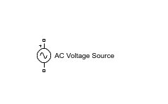
AC voltage source

Again, click on the search button, and then click on the search icon. In the search bar that will appear, type RLC, and a number of RLC branches will appear, as shown in the figure below.

RLC branch search

Select the series RLC branch, as we have in the above figure, and double-click on it to place the component in the Simulink window. The series RLC branch, when placed, is shown in the figure below.

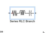
Series RLC branch

This branch can be converted to any of the three components or any combinations of the three components, i.e., R, L, C, RL, RC, and LC, etc. In our case, we need three components, i.e., R, L, and C, so we will place three such Series RLC branches on the Simulink window as shown in the figure below.

3 RLC branches

Selecting Branch

Now the question is: How do we convert these branches into individual components? Firstly, double-click on the first RLC branch, and a parameters window will appear. There will be a menu to select which combination of all three components we want to place on our Simulink window. From that menu, select R to convert the series RLC branch to a resistor branch, as shown in the figure below.

Resistor branch in RLC circuit

Resistor branch

Similarly, we repeat this process with the second branch, but this time we select the inductor option from the menu, as shown in the figure below.

Inductor branch of RLC circuit

Inductor branch

Lastly, we do the same with the third branch, but this time select the capacitor option from the menu, as shown in the figure below.

Capacitor branch of RLC circuit

Capacitor branch

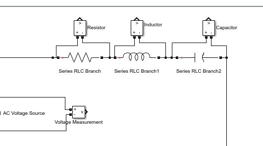
The three branches will then be converted to three different components, i.e., resistor, capacitor, and inductor, as shown in the figure below.

Changed branches of RLC circuit

Changed branches

Now we want to place a voltage measurement device, which will help us measure the voltage at each node of the circuit. In the search bar, type voltage measurement, as shown in the figure below.

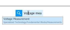
Voltage measurement search

RLC circuit

Connect the voltage measurement block at the ends of the AC input source and connect all the branches to complete the loop as in the following figure below.

Connected RLC circuit

Connected circuit

Now in the search bar, type ground, and a number of grounds will appear. Refer to the figure below.

Ground search

Connect the ground to the negative side of the AC voltage source, as shown in the figure below.

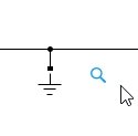
Connected ground

Place three other voltage sources from the same search bar and connect each of them across each of the components connected previously, i.e., the resistor, inductor, and capacitor, as shown in the figure below.

Voltage measurement

Now, from the library browser’s commonly used blocks section, select a scope, as shown in the figure below.

Scope placement

Place four such scopes and connect each of them with the voltage measurement devices as shown in the figure below.

Connected scopes to RLC circuit

Connected scopes

By doing so, we will not be able to see all the waveforms simultaneously. However, there is another option. We can give all the inputs to the same scope by adjusting the properties of the scope. Double-click on the scope, and from the window thus obtained, select the configuration properties button as shown in the figure below.

Configuration properties

From the properties, change the number of input ports from 1 to 4, as shown in the figure below.

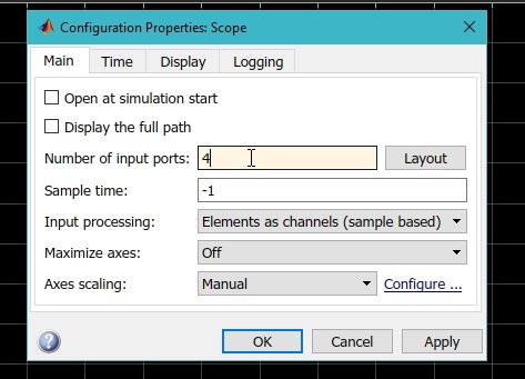
Input ports

Simulink Model

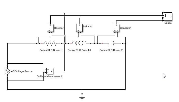
Connect the nodes of each of the voltage measuring devices to the inputs of the scope, as we can see in the following figure.

Multiple input scope

This block diagram will not run, however, because the power blocks are not initialized. We need to place a Power GUI block in the diagram to make it error-free. Search “powergui” in the search bar, as shown in the figure below.

Powergui search

Place the block anywhere in the block diagram, as shown in the figure below.

Powergui

Simulation

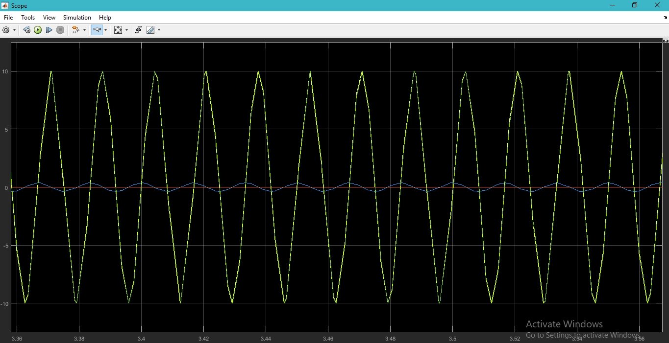
Run the block diagram and double-click on the scope to see the output of the waveforms, as shown in the figure below.

Output of RLC circuit

Output

Click on the view button and check the legends option, as shown in the figure below.

Legends

To display all four graphs separately, click on the arrow at the side of the settings button and select layout as shown in the figure below.

Layout

Select four blocks from the layout window, as shown in the figure below.

Layout blocks of RLC circuit

Layout blocks

This will show all the graphs in separate sections. Scale all the graphs according to need, as shown in the figure below.

Output graphs of RLC circuit

Output graphs

Notice the amplitude of all the waveforms, which are in accordance with the theory.

Exercise

Try to work with RL and RC circuits. Use the same fashion as discussed here, except use either an inductor or a capacitor in place of both.

Conclusion

In conclusion, this tutorial provides an in-depth overview of designing and simulating RLC circuits using Simulink. It covers step-by-step procedures along with an explanation of an example to help us better understand the concept. You can use this to design more complex and advanced filter circuits. At last, we have provided an example to reinforce the concept of this tutorial. Hopefully, this was helpful in expanding your knowledge of designing using Simulink.