Scientific Journal and Sci-Fi Themed Color Palettes for ggplot2 (original) (raw)
Discrete color palettes
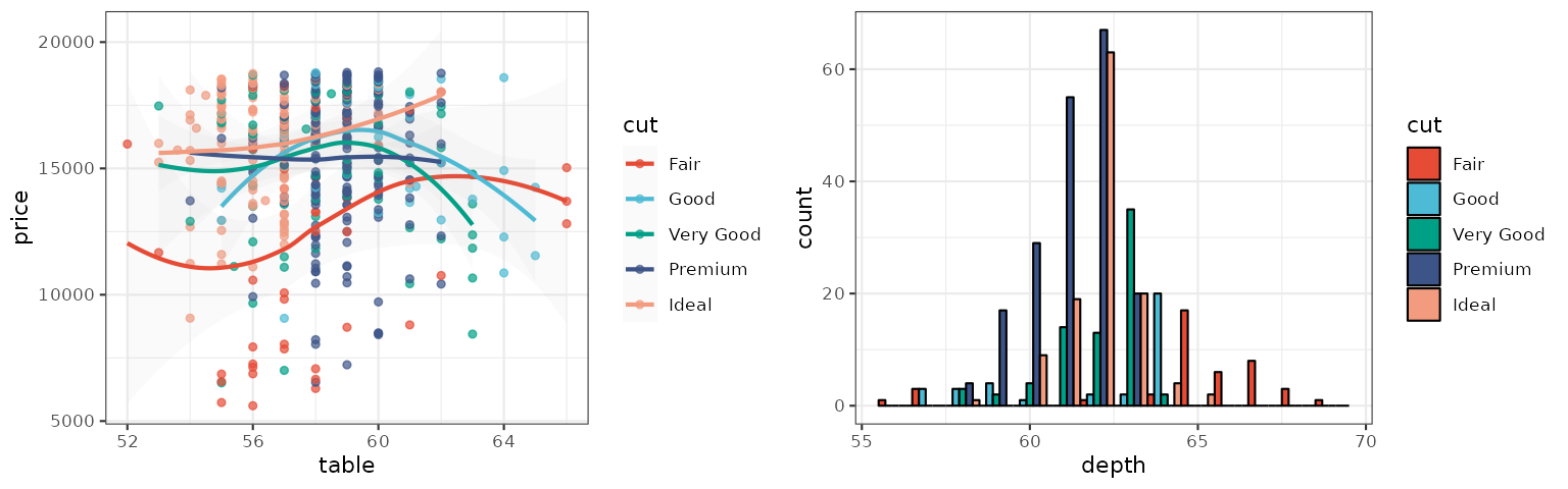
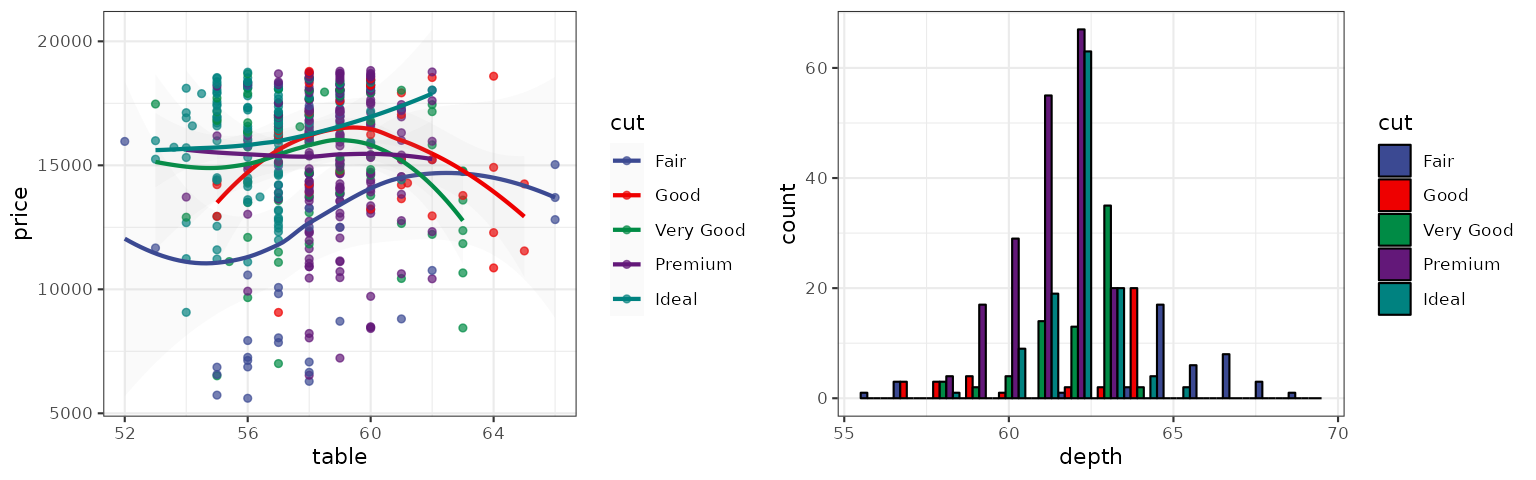
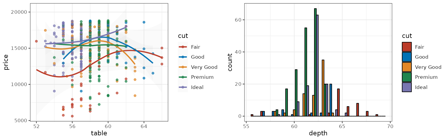
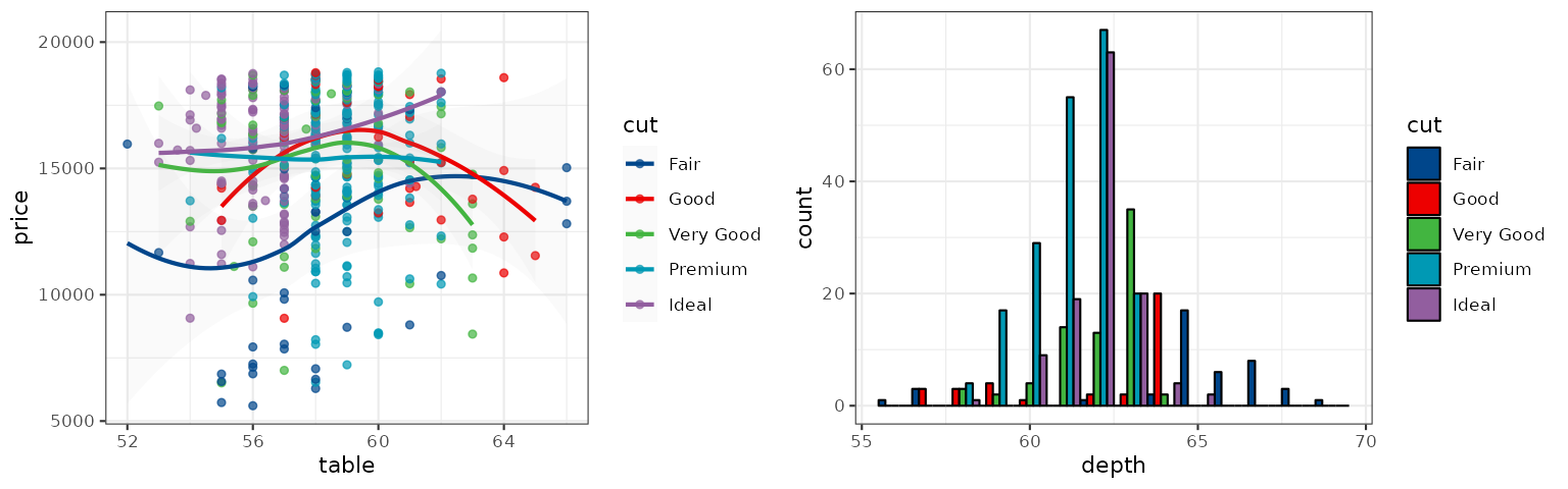
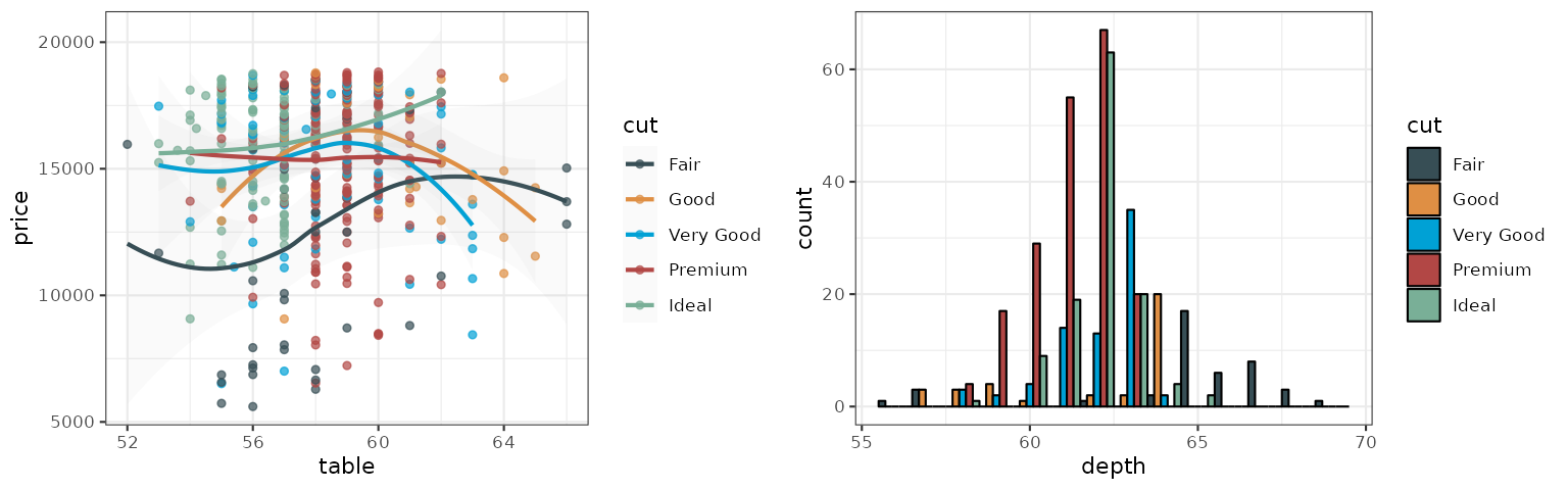
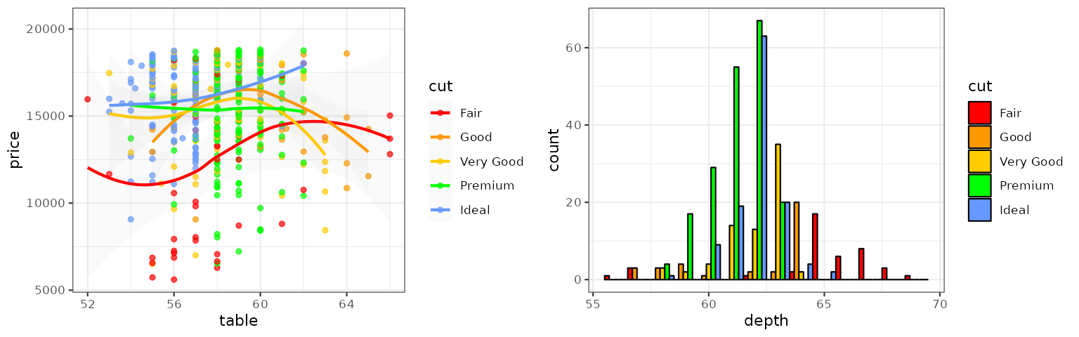
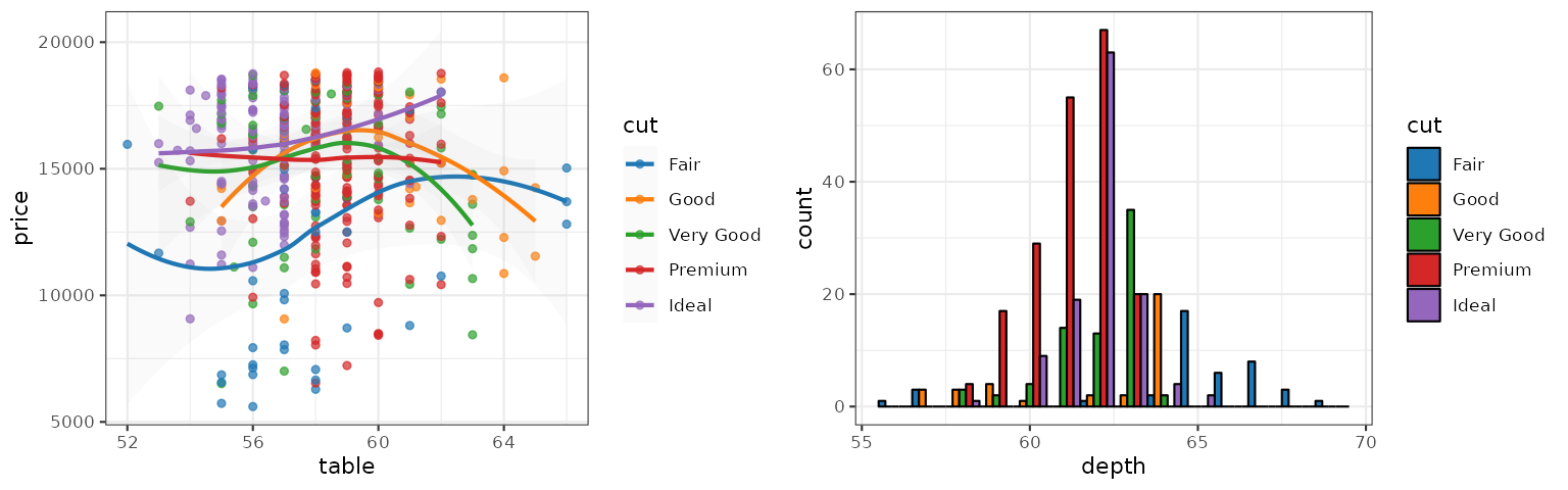
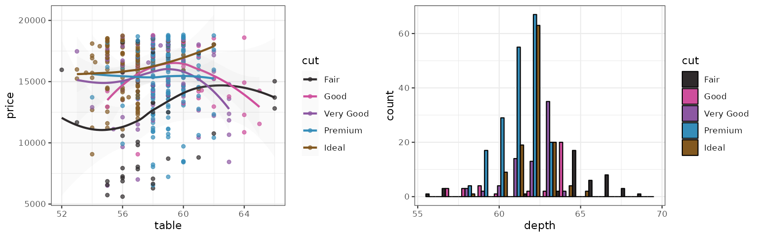
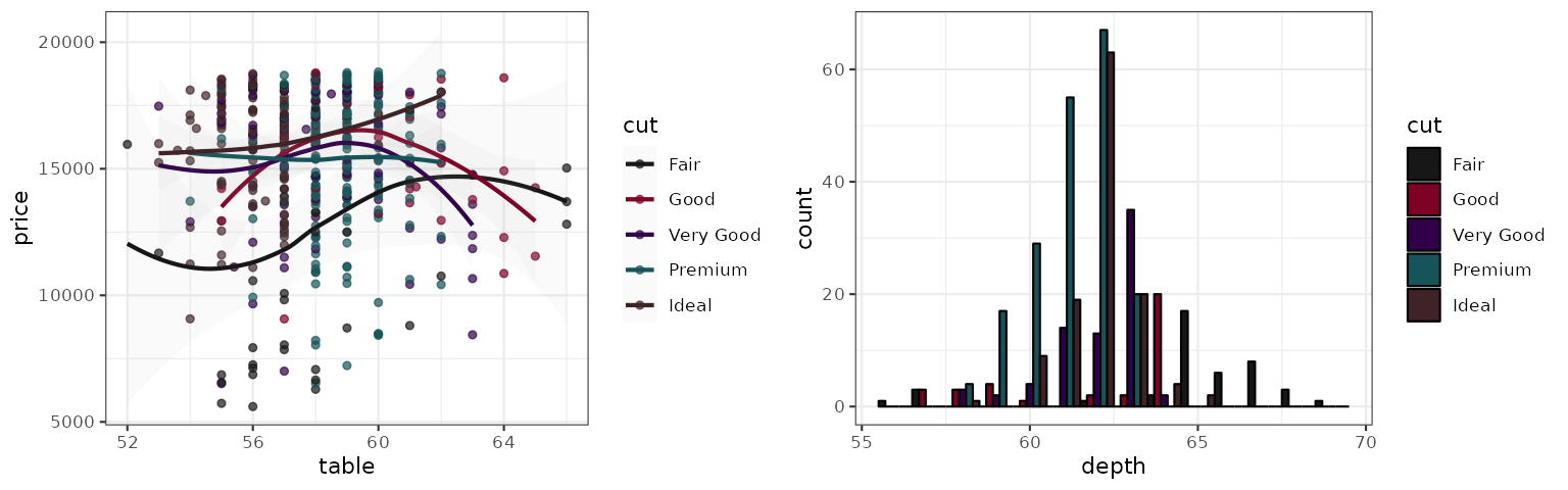
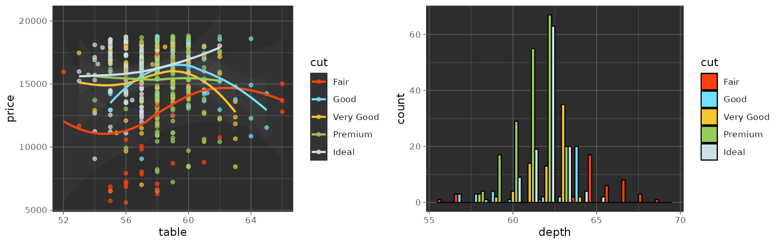
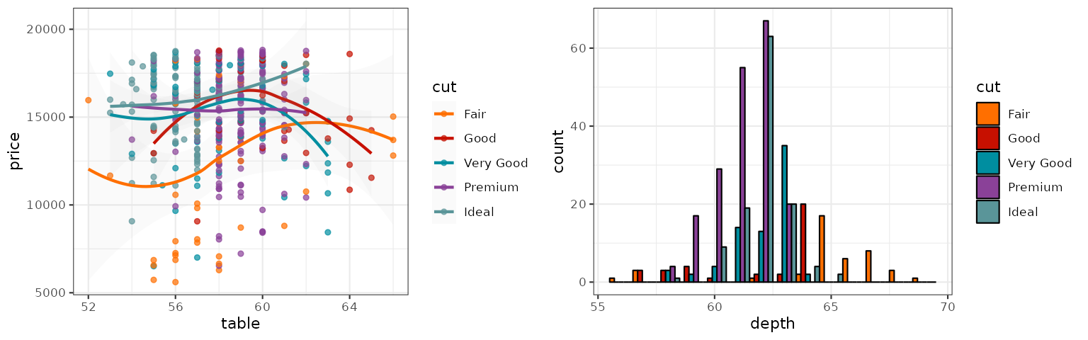
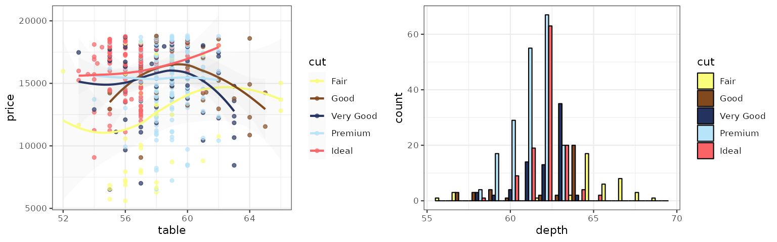
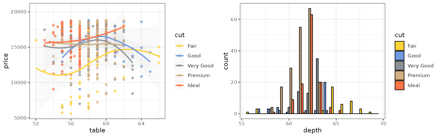
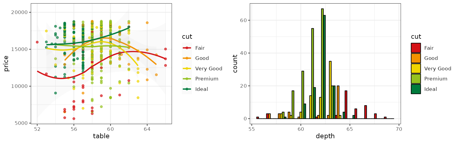
We will use scatterplots with smooth curves, and bar plots to demonstrate the discrete color palettes in ggsci.
library("ggsci")
library("ggplot2")
library("gridExtra")

data("diamonds")

p1 <- ggplot(
  subset(diamonds, carat >= 2.2),
  aes(x = table, y = price, colour = cut)
) +
  geom_point(alpha = 0.7) +
  geom_smooth(method = "loess", alpha = 0.05, linewidth = 1, span = 1) +
  theme_bw()

p2 <- ggplot(
  subset(diamonds, carat > 2.2 & depth > 55 & depth < 70),
  aes(x = depth, fill = cut)
) +
  geom_histogram(colour = "black", binwidth = 1, position = "dodge") +
  theme_bw()
NPG
The NPG palette is inspired by the plots in the journals published by Nature Publishing Group:
AAAS
The AAAS palette is inspired by the plots in the journals published by American Association for the Advancement of Science:
NEJM
The NEJM palette is inspired by the plots in the New England Journal of Medicine:
Lancet
The Lancet palette is inspired by the plots in _Lancet_journals, such as Lancet Oncology:
JAMA
The JAMA palette is inspired by the plots in the Journal of the American Medical Association:
JCO
The JCO palette is inspired by the the plots in Journal of Clinical Oncology:
UCSCGB
The UCSCGB palette is from the colors used by UCSC Genome Browser for representing chromosomes. This palette (interpolated, with alpha) is intensively used in visualizations generated by Circos.
D3
The D3 palette is from the categorical colors used by D3.js (version 3.x and before). There are four palette types (category10, category20,category20b, category20c) available.

LocusZoom
The LocusZoom palette is based on the colors used by LocusZoom.
IGV
The IGV palette is from the colors used by Integrative Genomics Viewer for representing chromosomes. There are two palette types (default, alternating) available.
UChicago
The UChicago palette is based on the colors used by the University of Chicago. There are three palette types (default, light, dark) available.
Star Trek
This palette is inspired by the (uniform) colors in Star Trek:
Tron Legacy
This palette is inspired by the colors used in Tron Legacy. It is suitable for displaying data when using a dark theme:
Futurama
This palette is inspired by the colors used in the TV show_Futurama_:
Rick and Morty
This palette is inspired by the colors used in the TV show Rick and Morty:

The Simpsons
This palette is inspired by the colors used in the TV show The Simpsons:
Frontiers
This color palette inspired by Frontiers:

Continuous color palettes
There are two types of continuous color palettes in ggsci: diverging and sequential. Diverging palettes have a central neutral color and contrasting colors at the ends, making them suitable for visualizing data with a natural midpoint. Sequential palettes use a gradient of colors that range from low to high intensity or lightness, making them ideal for representing data with increasing or decreasing values.
We will use a correlation matrix visualization (a special type of heatmap) to demonstrate the diverging color palettes.
To demonstrate sequential palettes, we use a random matrix:
set.seed(42)
k <- 6
x <- diag(k)
x[upper.tri(x)] <- runif(sum(1:(k - 1)), 0, 1)
x_melt <- data.frame(
  Var1 = rep(seq_len(nrow(x)), times = ncol(x)),
  Var2 = rep(seq_len(ncol(x)), each = nrow(x)),
  value = as.vector(x)
)

p4 <- ggplot(x_melt, aes(x = Var1, y = Var2, fill = value)) +
  geom_tile(colour = "black", linewidth = 0.3) +
  scale_x_continuous(expand = c(0, 0)) +
  scale_y_continuous(expand = c(0, 0)) +
  theme_bw() +
  theme(
    legend.position = "none", plot.background = element_blank(),
    axis.line = element_blank(), axis.ticks = element_blank(),
    axis.text.x = element_blank(), axis.text.y = element_blank(),
    axis.title.x = element_blank(), axis.title.y = element_blank(),
    panel.background = element_blank(), panel.border = element_blank(),
    panel.grid.major = element_blank(), panel.grid.minor = element_blank()
  )
GSEA
The GSEA palette (continuous) is inspired by the heatmaps generated by GSEA GenePattern.

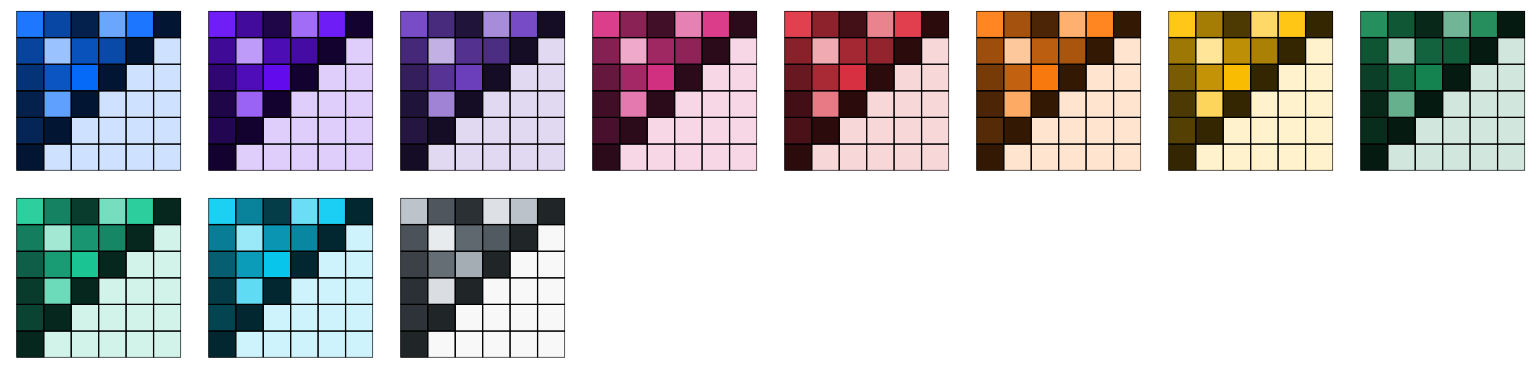
Bootstrap 5
The Bootstrap 5 color palettes are from the Bootstrap 5 color system.
grid.arrange(
  p4 + scale_fill_bs5("blue"), p4 + scale_fill_bs5("indigo"),
  p4 + scale_fill_bs5("purple"), p4 + scale_fill_bs5("pink"),
  p4 + scale_fill_bs5("red"), p4 + scale_fill_bs5("orange"),
  p4 + scale_fill_bs5("yellow"), p4 + scale_fill_bs5("green"),
  p4 + scale_fill_bs5("teal"), p4 + scale_fill_bs5("cyan"),
  p4 + scale_fill_bs5("gray"),
  ncol = 8
)
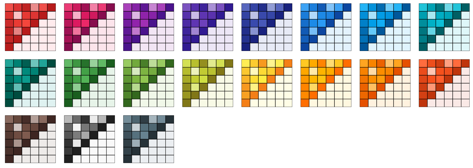
Material Design
The Material Design color palettes are from the Material Design color system.
grid.arrange(
  p4 + scale_fill_material("red"), p4 + scale_fill_material("pink"),
  p4 + scale_fill_material("purple"), p4 + scale_fill_material("deep-purple"),
  p4 + scale_fill_material("indigo"), p4 + scale_fill_material("blue"),
  p4 + scale_fill_material("light-blue"), p4 + scale_fill_material("cyan"),
  p4 + scale_fill_material("teal"), p4 + scale_fill_material("green"),
  p4 + scale_fill_material("light-green"), p4 + scale_fill_material("lime"),
  p4 + scale_fill_material("yellow"), p4 + scale_fill_material("amber"),
  p4 + scale_fill_material("orange"), p4 + scale_fill_material("deep-orange"),
  p4 + scale_fill_material("brown"), p4 + scale_fill_material("grey"),
  p4 + scale_fill_material("blue-grey"),
  ncol = 8
)
Tailwind CSS
The Tailwind CSS color palettes are from the Tailwind default colors.
grid.arrange(
  p4 + scale_fill_tw3("slate"), p4 + scale_fill_tw3("gray"),
  p4 + scale_fill_tw3("zinc"), p4 + scale_fill_tw3("neutral"),
  p4 + scale_fill_tw3("stone"), p4 + scale_fill_tw3("red"),
  p4 + scale_fill_tw3("orange"), p4 + scale_fill_tw3("amber"),
  p4 + scale_fill_tw3("yellow"), p4 + scale_fill_tw3("lime"),
  p4 + scale_fill_tw3("green"), p4 + scale_fill_tw3("emerald"),
  p4 + scale_fill_tw3("teal"), p4 + scale_fill_tw3("cyan"),
  p4 + scale_fill_tw3("sky"), p4 + scale_fill_tw3("blue"),
  p4 + scale_fill_tw3("indigo"), p4 + scale_fill_tw3("violet"),
  p4 + scale_fill_tw3("purple"), p4 + scale_fill_tw3("fuchsia"),
  p4 + scale_fill_tw3("pink"), p4 + scale_fill_tw3("rose"),
  ncol = 8
)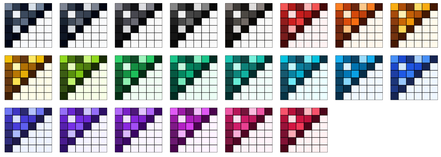
From the figure above, we can see that even though an identical matrix was visualized by all plots, some palettes are more preferable than the others because our eyes are more sensitive to the changes of their saturation levels.
Non-ggplot2 graphics
To apply the color palettes in ggsci to other graphics systems (such as base graphics and lattice graphics), simply use the palette generator functions in the table above. For example:
mypal <- pal_npg("nrc", alpha = 0.7)(9)
mypal
#> [1] "#E64B35B2" "#4DBBD5B2" "#00A087B2" "#3C5488B2" "#F39B7FB2" "#8491B4B2"
#> [7] "#91D1C2B2" "#DC0000B2" "#7E6148B2"

scales::show_col(mypal)
You will be able to use the generated hex color codes for such graphics systems accordingly. The transparent level of the entire palette is easily adjustable via the argument "alpha" in every generator or scale function.
Discussion
Please note some of the palettes might not be the best choice for certain purposes, such as color-blind safe, photocopy safe, or print friendly. If you do have such considerations, you might want to check out color palettes like ColorBrewer and viridis.
The color palettes in this package are solely created for research purposes. The authors are not responsible for the usage of such palettes.