Dynamic Charts Using Dynamic Arrays (original) (raw)
Thursday, March 25, 2021
Peltier Technical Services, Inc., Copyright © 2025, All rights reserved.
I recently wrote Dynamic Array Histogram, a tutorial showing how to build a histogram with a normal curve overlay. It worked great, except that the chart was hard-coded to the worksheet ranges with the data. When I changed the Dynamic Array formulas, the spill ranges changed size, and I had to manually adjust the chart data ranges. Not too big a deal for just a few series, but still an inconvenience.
Dynamic Array with One Column
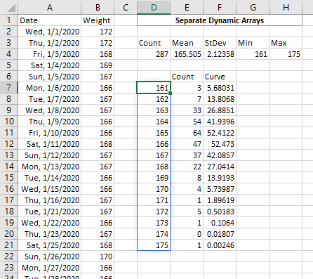
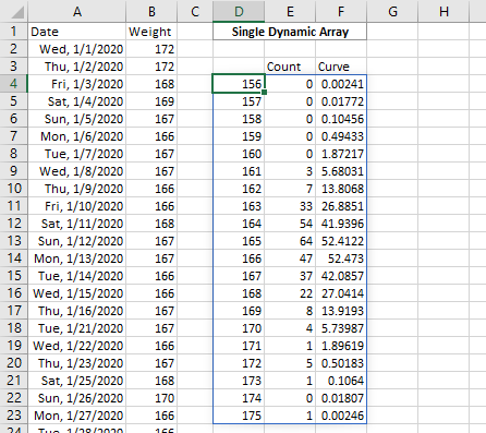
Here is what the data looks like. Cell D7 contains the following formula, which spills the numbers from 161 to 175 into the highlighted range D7:D21.
=SEQUENCE(H4+1-G4,1,G4,1)
I’ve written many tutorials about Dynamic Charts (see the list at the end of this article). Ordinarily I would generate some Names (aka dynamic range names) using a formula like this
=OFFSET(Sheet1!$D$6,1,0,COUNT(Sheet1!$D$6:$D$100),1)
then add the Names to the chart.
But we don’t need to use an OFFSET or other function to determine the size of the range of data. It’s a Dynamic Array, which we can reference using a hash sign (#): The entire spill range of the Dynamic Array formula in D7 is referenced by D7#.
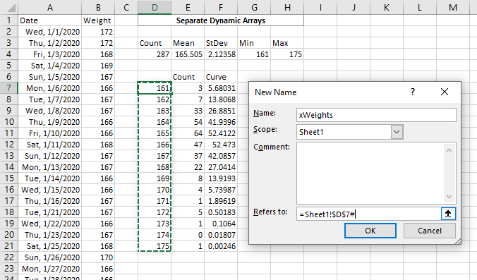
We still need to use Names in the dynamic chart, so click Define Name on Excel’s Formulas tab, give our Name a good name (xWeights), for Scope select Sheet1, and use =Sheet1!$D$7# as the Refers To formula. If you click in the Name textbox and back in the Refers To box, the range defined by the formula will be highlighted as shown.
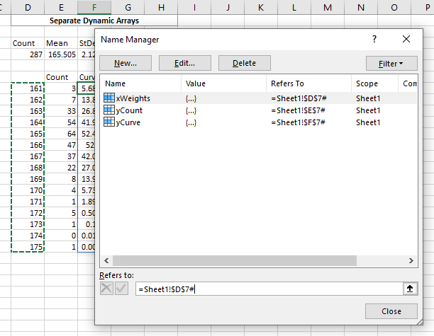
Similarly we had Dynamic Array formulas in cells E7 and F7, which spilled into E7# and F7#. We define Names yCount and yCurve using =Sheet1!$E$7# and =Sheet1!$F$7#. These are the Names we will use in our dynamic chart.
Press Ctrl+F3 to open the Name Manager and see all of the Names. As above, clicking in the Refers To box will highlight the range defined by the formula.
A note about naming Names. I use a prefix of x or y for chart data which will be used as X or Y values. I used to use a prefix of cht, but a fluky behavior in Excel 2007 and more recent versions changed that. If the name of a Name begins with R or C (think Row or Column), the name cannot easily be used in the series formula. If your language of Excel is not English, you can’t use the letters that the words for Row and Column begin with in your language.
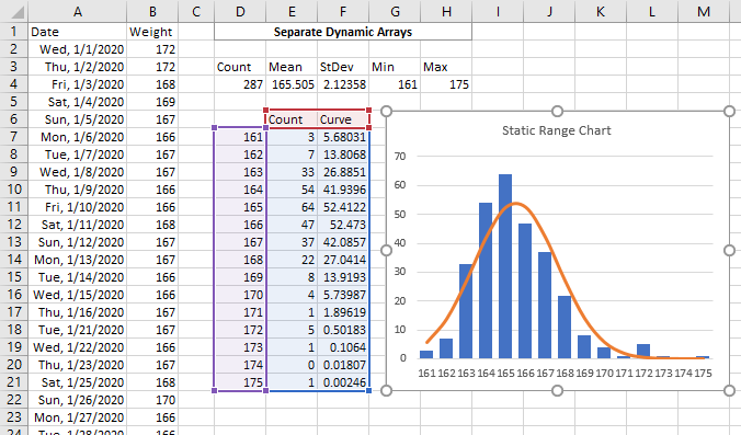
Start by selecting the range of data (D6:F21), including the header row. And note that the top left cell D7 is blank, to help Excel determine that the first column is X values. Insert a column chart, then right click on the Curve series, choose Change Series Chart Type, and select a line style.
When the chart is selected, the data range is highlighted.
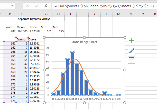
Select the Count series (the blue columns). The data is highlighted, and this SERIES formula appears in the formula bar.
=SERIES(Sheet1!$E$6,Sheet1!$D$7:$D$21,Sheet1!$E$7:$E$21,1)
This means the series name is in Sheet1!$E$6, the X values are in Sheet1!$D$7:$D$21, the Y values are in Sheet1!$E$7:$E$21, and it is the first series in the chart.
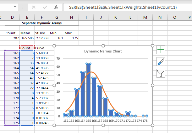
Right in the formula bar, change Sheet1!$D$7:$D$21 to Sheet1!xWeights and Sheet1!$E$7:$E$21 to Sheet1!yCount. Click Enter, so the SERIES formula becomes
=SERIES(Sheet1!$E$6,Sheet1!xWeights,Sheet1!yCount,1)
The worksheet data is still highlighted.
Repeat the procedure with the Curve series, changing the formula from
=SERIES(Sheet1!$F$6,Sheet1!$D$7:$D$21,Sheet1!$F$7:$F$21,2)
to
=SERIES(Sheet1!$F$6,Sheet1!xWeights,Sheet1!yCurve,2)
Dynamic Array with Multiple Columns
In the Dynamic Array Histogram tutorial, I showed how to make a multiple-column Dynamic Array from a single formula. This makes defining our Names more complicated, but only slightly so.
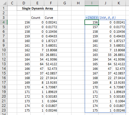
The Dynamic Array formula in cell D4 spills into multiple rows and columns.
The formula =D4# (entered into cell I4) spills into the same size range.

But I can use INDEX to return a portion of the Dynamic Array in D4#. For example, INDEX(D4#,1,1) returns the cell in the first row and first column of D4#.
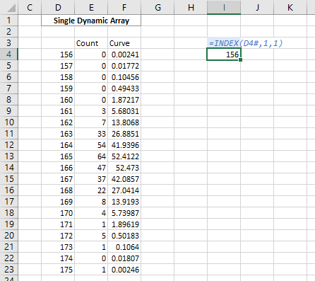
To get the first column, I specify the row as zero, in INDEX(D4#,0,1). I could leave out the zero altogether as long as I have the right amount of commas: INDEX(D4#,,1).

If I’d wanted just the first row, I use zero (or a blank) for the column index: INDEX(D4#,1,0) or INDEX(D4#,1,).

As it turns out, I could use INDEX(D4#,0,0) or INDEX(D4#,,) to reference the entire array.
I define my Names as above, name: xWeights, scope: Sheet2, refers to: =INDEX(Sheet2!$D$4#,0,1).
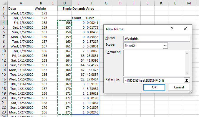
Define yCount and yCurve as =INDEX(Sheet2!$D$4#,0,1) and =INDEX(Sheet2!$D$4#,0,1), create and format the chart, and plug in the Names for the hard-coded addresses.
Update: Dynamic Charts Without Names
A year or so after I posted this article, Microsoft released an enhancement to Excel that made Dynamic-Array-driven charts themselves dynamic. If all of the data in the chart comes from a single Dynamic Array formula, the chart’s source data will change size to match the Dynamic Array’s spill range. This means we can select the original Dynamic Array and insert our chart, ignore the need to create Names for the X and Y values, and the chart will dynamically change its source data range as the Dynamic Array changes.
Here are more articles on the Peltier Tech blog that talk about dynamic charts.
- Dynamic Charts
- Easy Dynamic Charts Using Lists or Tables
- Dynamic Charts in Excel 2016 for Mac
- Dynamic Chart using Pivot Table and Range Names
- Dynamic Chart using Pivot Table and VBA
- Dynamic Ranges to Find and Plot Desired Columns
- Split Data Range into Multiple Chart Series without VBA
- VBA to Split Data Range into Multiple Chart Series
- Dynamic Chart Source Data (VBA)
- Dynamic Chart with Multiple Series
- Display One Chart Dynamically and Interactively
More Histogram Articles on Peltier Tech Blog
- Histogram With Normal Curve Overlay
- Histograms Using Excel XY Charts
- Histogram Using XY and/or Area Charts
- Filled Histograms Using Excel XY-Area Charts
- Histogram on a Value X Axis
- Histogram with Actual Bin Labels Between Bars
- Peltier Tech Histogram
More About Dynamic Arrays, LET, and LAMBDA
- ISPRIME Lambda Function
- Lambda Moving Average Formulas
- Improved Excel Lambda Moving Average
- Excel Lambda Moving Average
- LAMBDA Function to Build Three-Tier Year-Quarter-Month Category Axis Labels
- Calculate Nice Axis Scales with LET and LAMBDA
- VBA Test for New Excel Functions
- Dynamic Arrays, XLOOKUP, LET – New Excel Features