GlobPlot: exploring protein sequences for globularity and disorder (original) (raw)
Abstract
A major challenge in the proteomics and structural genomics era is to predict protein structure and function, including identification of those proteins that are partially or wholly unstructured. Non-globular sequence segments often contain short linear peptide motifs (e.g. SH3-binding sites) which are important for protein function. We present here a new tool for discovery of such unstructured, or disordered regions within proteins. GlobPlot (http://globplot.embl.de) is a web service that allows the user to plot the tendency within the query protein for order/globularity and disorder. We show examples with known proteins where it successfully identifies inter-domain segments containing linear motifs, and also apparently ordered regions that do not contain any recognised domain. GlobPlot may be useful in domain hunting efforts. The plots indicate that instances of known domains may often contain additional N- or C-terminal segments that appear ordered. Thus GlobPlot may be of use in the design of constructs corresponding to globular proteins, as needed for many biochemical studies, particularly structural biology. GlobPlot has a pipeline interface—GlobPipe—for the advanced user to do whole proteome analysis. GlobPlot can also be used as a generic infrastructure package for graphical displaying of any possible propensity.
INTRODUCTION
In the post-genomic era, discovery of novel domains and functional sites in proteins is of growing importance. A key part of initiatives like structural genomics is to optimise target selection by identifying domains and thereby increase spanning of fold and structure space (1). In addition, it has recently been recognised that many functionally important protein segments lie outside of globular domains in regions that are intrinsically disordered (2). Computational tools to help discern domains from intra-domain regions are key to such efforts. We describe here a graphical tool GlobPlot and a pipeline companion GlobPipe that do just this: they measure and display the propensity of protein sequences to be ordered or disordered.
There are many methods, such as SMART (Simple Modular Architecture Research Tool) (3), PRODOM (4), Pfam (5,6), PROSITE (7) and ELM (Eukaryotic Linear Motif, http://elm.eu.org) (8), available for finding globular domains (e.g. SH3, TyrKc, active sites) and linear motifs (e.g. SH3 ligands, LXXLL nuclear receptor ligands, tyrosine phosphorylation sites, post-translational modification sites) within a protein sequence. These methods typically rely on sequence similarity models, looking for recurrence of known domains or motifs by such means as HMMs (Hidden Markov Models) (9), pattern discovery (http://www.cs.ucr.edu/~stelo/pattern.html) or SW(Smith-Waterman)-profiles (10). Although these methods are of great value in annotating protein sequences, they are limited in their ability to uncover new features not yet discovered.
A complementary approach to domain or feature discovery is to predict protein structure, though such methods are computationally intensive, error prone and are usually designed to predict structure only within globular regions.
In order to predict possible targets for further structural analysis, we present here a method complementary to structure prediction. We describe a simple, easy to use, propensity/scale based tool for exploring both potential globular and disordered/flexible regions in proteins based on their sequence.
Protein disorder can be described as the lack of regular secondary structure and a high degree of flexibility in the polypeptide chain (2). Ordered regions are often termed globular and typically contain regular secondary structures packed into a compact globule. However no general definition of disorder exists.
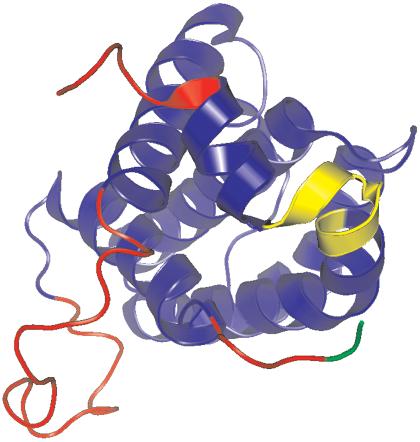
Disordered regions can contain functional sites, predicted as linear motifs by ELM and they are of growing interest owing to the increasing number of reports of intrinsically unstructured/disordered proteins (IUPs). IUPs contain regions that are partially or completely unfolded/unstructured in the native in vivo state of the protein. More than 100 IUPs are known (2,11), including Tau (12), Prions (13), Bcl-2 (Fig. 1) and partially p53 (14). Although little is understood about the cellular and structural meaning of this state, it is thought that it may exist as a molten globule and become ordered only when bound to another molecule (15,16). It is clear, however, that IUPs play a central role in biology and in diseases mediated by protein misfolding and aggregation (17,18).
Figure 1.
GlobPlot predictions for human Bcl-2. The predicted disordered segments are mapped on the structure in red. The yellow helix kink is falsely predicted as a disordered segment. The green segment is not predicted by GlobPlot probably because the algorithm has lower sensitivity in the termini due to the Savitzky-Golay filter. Blue color corresponds to the globular domain of Bcl-2.
Prediction of disorder can currently be performed using SEG (19), which searches for regions of low sequence complexity. However, low complexity of the sequence does not imply disorder in all cases. It is also possible to use methods such as hydrophobicity plots, though this approach is better suited to identification of segments, such as transmembrane helices, rather than finding long segments of disorder.
PONDR (http://www.pondr.com) (20,21) is a neural network based tool for disorder prediction, but it is not freely accessible.
Prot-Scale (http://us.expasy.org/cgi-bin/protscale.pl) is a general resource for showing amino acid propensity scales, using a sliding window algorithm. Prot-Scale does not offer any dedicated disorder predictor.
We discuss here GlobPlot, a tool to identify regions of globularity and disorder within protein sequences. It is a simple approach based on a running sum of the propensity for amino acids to be in an ordered or disordered state. We show that, despite its simplicity, this method is able to identify such regions when compared to domain databases and sets of disordered proteins.
INSIDE GlobPlot
Propensity sets
At the heart of GlobPlot are propensities, P, for all amino acids to be in globular or non-globular states. The GlobPlot package currently contains seven different propensity sets, though others could easily be added. There is no standard definition of disorder and no large set of universally agreed disordered proteins. Moreover, different parts of proteins are probably ordered under different conditions. We have thus developed a tool that allows parameters from different definitions of disorder to be applied.
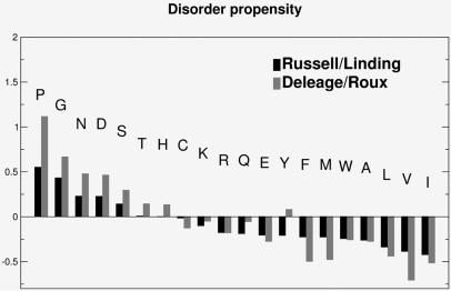
We designed parameters based on the hypothesis that the tendency for disorder can be expressed as _P_=RC_−_SS where RC and SS are the propensity for a given amino acid to be in ‘random coil’ and regular ‘secondary structure’, respectively. The starting point for the propensity scales were parameters for secondary structure and ‘random coil’ described by Chou and Fasman (22–24) and later introduced as propensities by Deleage and Roux (25). Initially, we defined a set solely based on these parameters (shown as Deleage/Roux in Fig. 2). However, we found that this scale performed poorly in finding disordered segments. Since the structure database is now much larger, we decided to recalculate propensities for amino acids to be either in regular secondary structures (α-helices or β-strands) defined by DSSP (26) or outside of them (‘random coil’, loops, turns etc.). We defined a non-redundant set of proteins by taking one representative from each superfamily in the SCOP database [version 1.59; http://scop.mrc-lmb.cam.ac.uk/scop/ (27,28)]. The frequencies RC and SS for each amino acid were calculated from this dataset. The resulting propensities, named Russell/Linding are given in Figure 2. Combining ‘random coil’ and ‘secondary structure’ in the Russell/Linding set enhanced the discrimination of the graphs and is the key factor in the success of this scale being able to detect both disorder and globular packing. GlobPlot is not intended as a competitor for secondary structure prediction. It cannot give the same level of detail as one can obtain from a secondary structure prediction based on a multiple alignment.
Figure 2.
Propensities for disorder/globularity detection. The Russell/Linding is the default set used by the GlobPlot algorithm.
We also calculated propensities based on coordinates described as missing from the protein databank (http://www.pdb.org) (29). We considered the same set of representatives, but here we ignored domain definitions (i.e. we took the whole chain or protein). We then looked for the ‘REMARK 465’ records in the associated PDB files (restricting these to the appropriate chain when required) for residues not seen either in the electron density or the NMR structure. We presumed this set to be disordered, and all residues with C-α entries to be ordered. The resulting propensity set named REMARK465 is online but still under development. The performance of this scale in predicting disorder will be evaluated in future work.
We provide a variety of different scales or propensities for the user to explore, the numerical values can be obtained from the link given in Table 1. In addition to the mentioned scales for finding disorder we also have some classical scales online for hydropathy.
Table 1. Additional online material.
The algorithm
The basic algorithm behind GlobPlot is simple and very fast. For each amino acid a, we have defined a propensity
(Fig. 2). Given a protein sequence of length L, we define a sum function Ω as follows:
where P(a i) is the propensity for the _i_th amino acid and ln is the natural logarithm.
We run a digital low-pass filter based on Savitzky-Golay (30) over Ω in order to smooth the curve and get the numerical estimation of the first order derivative. The filtering is performed by an external open source C module (sav_gol) from the TISEAN 2.1 (31) Nonlinear Time Series Analysis package (http://www.mpipks-dresden.mpg.de/~tisean/). The resulting smoothed function ΩS is plotted using the DISLIN 8.0 package. DISLIN is distributed as platform specific binaries from http://www.linmpi.mpg.de/dislin/. The ln(i+1) term was introduced in order to balance the plot more evenly between the N and C-terminal, doing so by increasing the weight of the terms as a function of residue number. Putative globular and disorder segments are selected using a simple peak finder algorithm (referred to as PeakFinder). The peaks are chosen when the first derivative shows positive (disorder) or negative (globular) values over a continuous stretch of the minimum length given by the user as ‘PeakFinder window length’.
We opted to use a running sum function for three reasons. Firstly, it results in plots that are easy to interpret, whether by human or algorithm. Secondly, it is a simple approach to a very complex problem. Thirdly, there is no dependency on frame length as is the case for sliding window methods such as SEG or Prot-Scale.
We expect that one could construct algorithms that avoid the unbalanced weighting of the residue numbers and work more directly on the propensities; we plan to incorporate this in later versions.
TESTING GlobPlot
Benchmarking methods to predict disorder are hampered by both the lack of a standard definition of disorder and the lack of a quality dataset. Performance of a particular set of parameters will clearly depend on the dataset from which they are derived. The benchmarking of GlobPlot was done using the GlobPipe script collection and SQL (structured query language) based data mining (we are using PostgreSQL as relational database). We found that SQL data mining is a very efficient, fast and flexible way of performing data analysis. We benchmarked GlobPlot by a variety of approaches:
- test of disorder prediction of IUPs;
- comparison to PONDR disorder prediction;
- structural (SMART) context analysis of predicted disordered segments;
- benchmarking prediction of globular segments (GlobDoms) versus SMART;
- benchmarking prediction of disorder using structural B-factors.
GlobPlot on IUPs
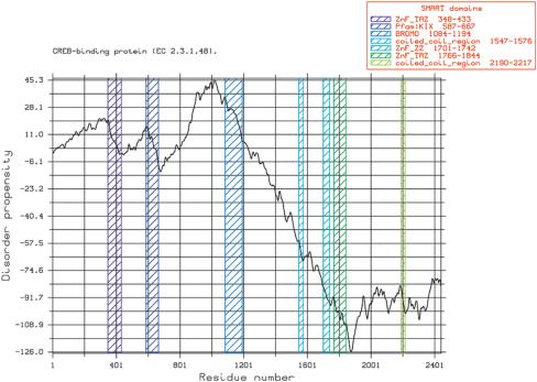
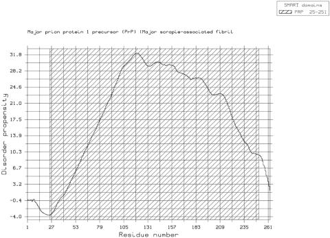
The operational definition of IUPs is based on X-ray, NMR, CD (circular dichroism) and a variety of hydrodynamic volume measurements. Several IUPs are only unstructured under certain equilibrium conditions where the unfolded state is favored over the folded/structured state (32). Formation of coiled-coil dimerisation provides a well understood example of such an equilibrium. Induced folding upon binding to a target protein is also observed as in the case of the proteins CREB and CBP (33,34). This indicates that IUP-assigned protein sets are error-prone and should be carefully considered on a case by case basis. We selected proteins from a recent review by Tompa [(11), Table 1]. We applied GlobPlot to the 20 proteins listed and predicted non-globular segments in all of these proteins. The plots of these proteins can be viewed in the online GlobPlot gallery (http://globplot.embl.de/gallery/). We found that the CBP protein, rather than the CREB protein, shows significantly disordered regions (Fig. 3). In the case of FlgM it has recently been shown to be partially folded in vivo (32), the N-terminal part is correctly found by GlobPlot to be disordered. We suggest that Stathmin seems to be disordered because the interaction partner Tsg-101 is partially disordered. Finally the GlobPlot of the bovine prion protein shows clearly the N-terminal flexible tail found in the NMR study of this protein (Fig. 4).
Figure 3.
GlobPlot of human CREB binding protein (CBP_HUMAN). About half of the sequence appears to be in a disordered state with long flexible regions observed at N- and C-terminus. The flexible region just after the KIX domain might be important for induced binding of the pKID domain of CREB to CBP (33,34). For further discussion of disorder in CBP/CREB see Wright et al. (2).
Figure 4.
GlobPlot of bovine prion protein (P10279). The flexible N-terminal segment is easily spotted (13). The SMART ‘domain’ is, in this case, a protein signature not a descriptor of a globular fold. The plot was created by using the ‘Create PostScript’ option.
GlobPlot versus PONDR
A comparison of GlobPlot and the neural network predictor PONDR (http://www.pondr.com) (20,21) were severely hampered by the fact that the PONDR server only allows 30 predictions. Therefore we could only test qualitatively. In general, GlobPlot and PONDR predict about the same on the disordered proteins that we tested (Table 2).
Table 2. Comparison of GlobPlot and PONDR predictions.
| Protein | PONDR segment | GlobPlot segment | Comment |
|---|---|---|---|
| PRIO_BOVIN | 25–141 | 22–118, 133–141 | Effectively the same |
| Q13541 [4E-BP1] | 1–43, 62–116 | 24–49, 63–95, 97–106 | Effectively the same |
| PRP1_HUMAN | 15–331 | 28–322 | Effectively the same |
| TN101_HUMAN | 145–225 | 137–220 | Effectively the same |
| CA19_HUMAN | 256–402, 415–759, 777–902 | 260–471, 474–757, 782–903 | Effectively the same |
| Q9HBB5 [MUCDHL-FL] | 435–664, 730–786, 805–845 | 454–660,695–716, 723–768, 810–836 | Effectively the same |
| ROG_HUMAN | 84–130, 139–205, 348–391 | 87–200, 203–337, 342–382 | Different |
| K1CI_HUMAN | 344–384, 461–622 | 8–148, 460–613 | Different |
| O95060 [AblBP4] | 158–368 | 160–283, 293–307, 317–363, 375–385 | Effectively the same |
GlobDoms versus SMART
To determine to what extent GlobPipe can be used for isolation of putative globular domains (GlobDoms) we benchmarked against the SMART server (http://smart.embl.de). A data set of 10 497 human protein sequences was created. The following criteria were imposed on the candidate sequences:
- subset of SWISS-PROT human proteome that contains SMART hit(s) (Ivica Letunic, personal communication);
- key word filtered for ‘fragments’, ‘putative’, ‘hypothetical’ and ‘similar to’;
- non-redundant data (based on EMBLs nrsp95).
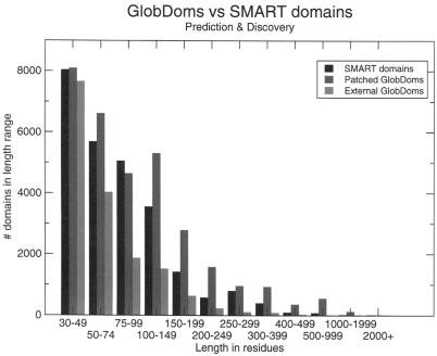
The results of the structural context analysis can be seen in Figure 5. In the 10 497 proteins SMART predicted 47 340 domains, of which 25 672 were longer than 30 residues. Finally 47 989 putative globular domains (GlobDoms) were found by GlobPipe using a PeakFinder search window of length 30. GlobPlot predicts a substantial fraction of putative domains that are not known to/found by SMART/Pfam.
Figure 5.
Benchmarking of GlobDoms versus SMART domains. We used the GlobPipe PeakFinder to search for ‘down-hill’ areas (negative first order derivative) in the GlobPlot graph. Assuming that such regions (GlobDoms) can be patched together (and thereby define a single domain), if they overlap with or are completely embedded in a SMART domain on the same sequence, we establish a recovery of the SMART domains. Patched GlobDoms are predicted domains co-located with a known SMART domain on the same sequence. The green ‘Discovery’ bar shows how many GlobDoms are found entirely outside SMART predictions. From fragments of length ≥100, we observe that the fraction originating from the overlapped segments results in overprediction.
The PeakFinder module was modified to find ‘downhill’ areas in the GlobPlot that were 30+ amino acids. Thirty is about the minimum size that SMART annotation will consider a globular domain (except for disulfide linked mini-domains).
Disordered segments in SMART context
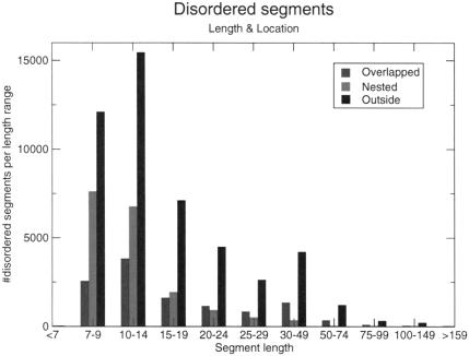
We also made an attempt to look for the structural context of the disordered segments GlobPipe predicted in the above dataset. GlobPipe predicted 75 152 disordered segments using an eight residue long frame for the smoothing routine. We compared all of these segments with the domain architecture of the ‘host sequence’ as predicted by SMART. We found that most flexible regions fall outside globular domains (Fig. 6). For short peptides (7–14 residues) ∼50% are nested within SMART domains, for longer segments much fewer are nested and more are overlapping. We interpret these data as an indication that GlobPlot does seem to discriminate structural features and context of the disordered segments. Another observation is that most segments are within this short range, from a functional point of view this makes sense since we know that most functional flexible/disordered sites are of length 5–10. This gives a basis for deploying GlobPlot as a discovery/overview tool for the annotation of functional sites.
Figure 6.
Structural analysis of disordered segments. For all lengths of segments it is observed that more segments are found in sequence not predicted to be globular by SMART. However we observe a significant amount of internal disorder, which in many cases can correspond to a loop, hinge or another type of flexible insertion in the protein. The amount of overlapping is difficult to interpret, however we have observed that GlobPlot often predicts the domain boundaries more precisely than SMART does. This is because SMART typically uses only the ‘core’ sequences to define the Hidden Markov Model for a given domain.
Benchmarking using B-factors
Structural B-factors (isotropic temperature factors) were chosen because they are unrelated to the data we used in creating the propensity sets and because they, to a certain degree, reflect disorder and flexibility in the polypeptide chain (35–37). However, B-factors vary greatly between structures and are often influenced by crystal packing and other structural artefacts. In attempt to avoid these issues only the B-factor for the C-α atom was considered.
We defined a non-redundant set of proteins by taking one representative from each family in the SCOP database. The set was reduced to contain only X-ray structures of a resolution higher than 2.2 Å. The B-factor values were extracted from the PDB entries and the average B-factor and standard deviation was calculated for each chain. In order to have a stringent set, only residues that had a B-factor 3.5 standard deviations above the average were marked as disordered. The resulting data were then compared to the predictions of GlobPlot using the Russell/Linding propensity set. The seven most N- and C-terminal residues were ignored due to the lower sensitivity introduced by the Savitzky-Golay filtering.
At a specificity of 88% we obtained a sensitivity of 28%. Accounting for the low sensitivity was that 74% of the false negatives were due to high B-factor helix bundles and domains observed in enzymes (especially ligases, hydrolases and oxidoreductases) (38). We expect a putative sensitivity of 59% in this dataset.
A fundamental problem with benchmarking a disorder predictor is that currently no general definition of disorder is agreed on. Furthermore, we here describe disorder as two states (disorder/order), whereas one should expect it to be multistate. These issues makes it very difficult to select unbiased datasets for benchmarking.
We will continue the hunt for better datasets and further bench-marking to be used in disorder studies in future work. We iterate that GlobPlot successfully identifies the disorder in well char-acterised proteins like TAU, CBP, prions and PRP1_HUMAN.
USING GlobPlot
The GlobPlot software package consist of two parts, both implemented in the language Python 2.2 (http://www.python.org): GlobPlot and GlobPipe.
An Internet plotting server—GlobPlot
GlobPlot is a CGI (common gateway interface) based server accessible at http://globplot.embl.de, for exploring disorder and globular segments (GlobDoms).
The web interface is fairly straight forward to use, the user can paste a sequence or enter the SWISS-PROT/SWALL accession (eg. P08630) or entry code (e.g. BTLK_DROME). The GlobPlot server fetches the sequence and description of the polypeptide from an ExPASy server using Biopython.org software.
By default the server will send the sequence to the public SMART queue (http://smart.embl.de, that by default also predicts Pfam domains) and display any obtained domain predictions as colored boxes layered on the graph. The SMART/Pfam prediction substantially increases the plotting time, but is set to ‘on’ by default because it is a very informative feature. Showing the boundaries of known SMART domains in the sequence is of great value for navigating as well as analysing the globplot. The SMART predictions are used solely for graphical viewing, they are not used in the GlobPlot routine itself.
In order to present a graph that is smoothed for digital noise, we use a digital low-pass filter based on Savitzky-Golay (least square fitting). The user can obtain the non-smoothed curve, as well as change the window length used by the Savitzky-Golay algorithm, however normally the default settings for the smoothing are optimal. Further information on the available user options are described in Table 3. In order to give the user the possibility for further data analysis, the numerical data for the plot can be downloaded in tabulated format from the result page and used in other plotting software such as Grace, OpenOffice.org or Excel. Because GlobPlot is ‘scale stable’ the user can paste in a specific sub-sequence and obtain a zoomed plot. The output file format for the plot is PNG (portable network graphics), but publication quality plots can be created using the postscript option. Residue ranges for found disordered segments and globular regions (GlobDoms) are shown at the bottom of the output page.
Table 3. Non-trivial user options available.
| Name of option | Effect of option |
|---|---|
| Plot title | If a SWISS-PROT acc/entry is entered, an auto generated title is created. This option allows for an alternative title |
| Windowlength PeakFinder | The minimal length of continuous disorder the PeakFinder should select |
| Perform SMART prediction | Performs a domain search using SMART, slows down the plotting |
| Show d_y_/d_x_ plot | Shows the smoothed first order derivative of the sum function used by the PeakFinder to find segments of disorder |
| Show raw plot | Show the raw sum function without digital filtering |
| Window length for smoothing | The window length used by the least-square routine in the Savitzky-Golay filtering |
| Windowlength for derivative | Length of smoothing window used when calculating the first derivative |
| Propensity sets | The user can choose among several propensity sets |
A pipeline interface—GlobPipe
GlobPipe is a pipeline that can be used for proteome scale analysis. The pipeline software is not a complete package but rather a set of routines that performs tasks relevant for SQL driven data mining large amounts of data in a relational database (PostgreSQL, http://www.postgresql.org). GlobPipe is still under development but it should be possible for any user with some programming skills to set up their own pipeline analysis, using these routines. We expect to set up a database of disordered protein sequences based on GlobPipe predictions.
The GlobPlot/GlobPipe package
The full GlobPlot/GlobPipe package (excluding the DISLIN and TISEAN modules that both have to be obtained from their respective websites) can be downloaded as a tarball at http://globplot.embl.de/download.html. The software is released under the Academic Free License Version 1.2 and is thereby OSI Certified Open Source Software (http://www.opensource.org). The software has broad platform coverage and is currently served on a FreeBSD box.
GlobPlot CAN BE USED FOR …
- Finding regions that create trouble in your crystallisation setups.
- Searching for putative new globular domains and functional sites.
- Searching for IUPs and intrinsic disorder.
- Graphical visualisation of any propensity set that can be constructed for a polymeric sequence.
- Building a database of putative IUPs and domains using GlobPipe.
Acknowledgments
ACKNOWLEDGEMENTS
We thank Will Stanley, Kresten Lindorff-Larsen, Jesper Borg and David Martin for cool fruitful discussions and suggestions and Christine Gemuend and Ivica Letunic for SMART interface code/data. We are grateful to Francesca Diella, Chenna Ramu, Sophie Chabanis and Sara Quirk for reading this manuscript. This work was partly supported by EU grant QLRI-CT-2000-00127.
Finally we are deeply grateful to FreeBSD.org, (bio)Python.org, PostgreSQL.org, Debian.org and Apache.org for fantastic open free software.
REFERENCES
- 1.Brenner S. (2000) Target selection for structural genomics. Nat. Struct. Biol., 7 (suppl), 967–969. [DOI] [PubMed] [Google Scholar]
- 2.Wright P. and Dyson,H. (1999) Intrinsically unstructured proteins: re-assessing the protein structure-function paradigm. J. Mol. Biol., 293, 321–331. [DOI] [PubMed] [Google Scholar]
- 3.Letunic I., Goodstadt,L., Dickens,N., Doerks,T., Schultz,J., Mott,R., Ciccarelli,F., Copley,R., Ponting,C. and Bork,P. (2002) Recent improvements to the SMART domain-based sequence annotation resource. Nucleic Acids Res., 30, 242–244. [DOI] [PMC free article] [PubMed] [Google Scholar]
- 4.Servant F., Bru,C., Carrere,S., Courcelle,E., Gouzy,J., Peyruc,D. and Kahn,D. (2002) ProDom: automated clustering of homologous domains. Brief Bioinform., 3, 246–251. [DOI] [PubMed] [Google Scholar]
- 5.Mulder N., Apweiler,R., Attwood,T., Bairoch,A., Barrell,D., Bateman,A., Binns,D., Biswas,M., Bradley,P., Bork,P. et al. (2003) The InterPro Database, 2003 brings increased coverage and new features. Nucleic Acids Res., 31, 315–318. [DOI] [PMC free article] [PubMed] [Google Scholar]
- 6.Bateman A., Birney,E., Cerruti,L., Durbin,R., Etwiller,L., Eddy,S., Griffiths-Jones,S., Howe,K., Marshall,M. and Sonnhammer,E. (2002) The Pfam protein families database. Nucleic Acids Res., 30, 276–280. [DOI] [PMC free article] [PubMed] [Google Scholar]
- 7.Sigrist C., Cerutti,L., Hulo,N., Gattiker,A., Falquet,L., Pagni,M., Bairoch,A. and Bucher,P. (2002) PROSITE: a documented database using patterns and profiles as motif descriptors. Brief Bioinform., 3, 265–274. [DOI] [PubMed] [Google Scholar]
- 8.Puntervoll P., Linding,R., Gemünd,C., Chabanis-Davidson,S., Mattingsdal,M., Cameron,S., Martin,D.M.A., Ausiello,G., Brannetti,B., Costantini,A. et al. (2003) ELM server: a new resource for revealing short functional sites in modular eukaryotic proteins. Nucleic Acids Res., 31, 3625–3630. [DOI] [PMC free article] [PubMed] [Google Scholar]
- 9.Eddy S. (1998) Profile hidden Markov models. Bioinformatics, 14, 755–763. [DOI] [PubMed] [Google Scholar]
- 10.Smith T. and Waterman,M. (1981) Identification of common molecular subsequences. J. Mol. Biol., 147, 195–197. [DOI] [PubMed] [Google Scholar]
- 11.Tompa P. (2002) Intrinsically unstructured proteins. Trends Biochem. Sci., 27, 527–533. [DOI] [PubMed] [Google Scholar]
- 12.Schweers O., Schonbrunn-Hanebeck,E., Marx,A. and Mandelkow,E. (1994) Structural studies of tau protein and Alzheimer paired helical filaments show no evidence for betastructure. J. Biol. Chem., 269, 24290–24297. [PubMed] [Google Scholar]
- 13.Lopez Garcia F., Zahn,R., Riek,R. and Wuthrich,K. (2000) NMR structure of the bovine prion protein. Proc. Natl Acad. Sci. USA, 97, 8334–8339. [DOI] [PMC free article] [PubMed] [Google Scholar]
- 14.Kussie P., Gorina,S., Marechal,V., Elenbaas,B., Moreau,J., Levine,A. and Pavletich,N. (1996) Structure of the MDM2 oncoprotein bound to the p53 tumor suppressor transactivation domain. Science, 274, 948–953. [DOI] [PubMed] [Google Scholar]
- 15.Uversky V. (2002) Natively unfolded proteins: a point where biology waits for physics. Protein Sci., 11, 739–756. [DOI] [PMC free article] [PubMed] [Google Scholar]
- 16.Dunker A., Lawson,J., Brown,C., Williams,R., Romero,P., Oh,J., Oldfield,C., Campen,A., Ratliff,C., Hipps,K. et al. (2001) Intrinsically disordered protein. J. Mol. Graph. Model., 19, 26–59. [DOI] [PubMed] [Google Scholar]
- 17.Dunker A., Brown,C., Lawson,J., Iakoucheva,L. and Obradovic,Z. (2002) Intrinsic disorder and protein function. Biochemistry, 41, 6573–6582. [DOI] [PubMed] [Google Scholar]
- 18.Dunker A., Garner,E., Guilliot,S., Romero,P., Albrecht,K., Hart,J., Obradovic,Z., Kissinger,C. and Villafranca,J. (1998) Protein disorder and the evolution of molecular recognition: theory, predictions and observations. Pac. Symp. Biocomput., 473–484. [PubMed] [Google Scholar]
- 19.Wootton J. (1994) Non-globular domains in protein sequences: automated segmentation using complexity measures. Comput. Chem., 18, 269–285. [DOI] [PubMed] [Google Scholar]
- 20.Garner E., Cannon,P., Romero,P., Obradovic,Z. and Dunker,A. (1998) Predicting disordered regions from amino acid sequence: common themes despite differing structural characterization. Genome Inform Ser Workshop Genome Inform, 9, 201–213. [PubMed] [Google Scholar]
- 21.Garner E., Romero,P., Dunker,A., Brown,C. and Obradovic,Z. (1999) Predicting binding regions within disordered proteins. Genome Inform SerWorkshop Genome Inform, 10, 41–50. [PubMed] [Google Scholar]
- 22.Chou P. and Fasman,G. (1974) Conformational parameters for amino acids in helical, betasheet, and random coil regions calculated from proteins. Biochemistry, 13, 211–222. [DOI] [PubMed] [Google Scholar]
- 23.Chou P. and Fasman,G. (1978) Prediction of the secondary structure of proteins from their amino acid sequence. Adv. Enzymol. Relat. Areas Mol. Biol., 47, 45–148. [DOI] [PubMed] [Google Scholar]
- 24.Chou P. and Fasman,G. (1978) Empirical predictions of protein conformation. Annu. Rev. Biochem., 47, 251–276. [DOI] [PubMed] [Google Scholar]
- 25.Deleage G. and Roux,B. (1987) An algorithm for protein secondary structure prediction based on class prediction. Protein Eng., 1, 289–294. [DOI] [PubMed] [Google Scholar]
- 26.Kabsch W. and Sander,C. (1983) Dictionary of protein secondary structure: pattern recognition of hydrogen-bonded and geometrical features. Biopolymers, 22, 2577–2637. [DOI] [PubMed] [Google Scholar]
- 27.Lo Conte L., Brenner,S., Hubbard,T., Chothia,C. and Murzin,A. (2002) SCOP database in 2002: refinements accommodate structural genomics. Nucleic Acids Res., 30, 264–267. [DOI] [PMC free article] [PubMed] [Google Scholar]
- 28.Chandonia J., Walker,N., Lo Conte,L., Koehl,P., Levitt,M. and Brenner,S. (2002) ASTRAL compendium enhancements. Nucleic Acids Res., 30, 260–263. [DOI] [PMC free article] [PubMed] [Google Scholar]
- 29.Westbrook J., Feng,Z., Chen,L., Yang,H. and Berman,H. (2003) The Protein Data Bank and structural genomics. Nucleic Acids Res., 31, 489–491. [DOI] [PMC free article] [PubMed] [Google Scholar]
- 30.Press W.H. and Teukolsky,S.A. (2002) Numerical recipes. In Press, W.H. C++ The Art of Scientific Computing, 2nd Edn. Cambridge University Press. [Google Scholar]
- 31.Hegger R., Kantz,H. and Schreiber,T. (1999) Practical implementation of nonlinear time series methods: the TISEAN package. Chaos, 9, 413. [DOI] [PubMed] [Google Scholar]
- 32.Dedmon M., Patel,C., Young,G. and Pielak,G. (2002) FlgM gains structure in living cells. Proc. Natl Acad. Sci. USA, 99, 12681–12684. [DOI] [PMC free article] [PubMed] [Google Scholar]
- 33.Radhakrishnan I., Perez-Alvarado,G., Parker,D., Dyson,H., Montminy,M. and Wright,P. (1997) Solution structure of the KIX domain of CBP bound to the transactivation domain of CREB: a model for activator:coactivator interactions. Cell, 91, 741–752. [DOI] [PubMed] [Google Scholar]
- 34.Demarest S., Martinez-Yamout,M., Chung,J., Chen,H., Xu,W., Dyson,H., Evans,R. and Wright,P. (2002) Mutual synergistic folding in recruitment of CBP/p300 by p160 nuclear receptor coactivators. Nature, 415, 549–553. [DOI] [PubMed] [Google Scholar]
- 35.Parthasarathy S. and Murthy,M. (2000) Protein thermal stability: insights from atomic displacement parameters (B values). Protein Eng., 13, 9–13. [DOI] [PubMed] [Google Scholar]
- 36.Wampler J. (1997) Distribution analysis of the variation of B-factors of X-ray crystal structures; temperature and structural variations in lysozyme. J. Chem. Inf. Comput. Sci., 37, 1171–1180. [DOI] [PubMed] [Google Scholar]
- 37.Zoete V., Michielin,O. and Karplus,M. (2002) Relation between sequence and structure of HIV-1 protease inhibitor complexes: a model system for the analysis of protein flexibility. J. Mol. Biol., 315, 21–52. [DOI] [PubMed] [Google Scholar]
- 38.Rudino-Pinera E., Morales-Arrieta,S., Rojas-Trejo,S. and Horjales,E. (2002) Structural flexibility, an essential component of the allosteric activation in Escherichia coli glucosamine-6-phosphate deaminase. Acta Crystallogr. D Biol. Crystallogr., 58, 10–20. [DOI] [PubMed] [Google Scholar]
