A global reference for human genetic variation (original) (raw)
Abstract
The 1000 Genomes Project set out to provide a comprehensive description of common human genetic variation by applying whole-genome sequencing to a diverse set of individuals from multiple populations. Here we report completion of the project, having reconstructed the genomes of 2,504 individuals from 26 populations using a combination of low-coverage whole-genome sequencing, deep exome sequencing, and dense microarray genotyping. We characterized a broad spectrum of genetic variation, in total over 88 million variants (84.7 million single nucleotide polymorphisms (SNPs), 3.6 million short insertions/deletions (indels), and 60,000 structural variants), all phased onto high-quality haplotypes. This resource includes >99% of SNP variants with a frequency of >1% for a variety of ancestries. We describe the distribution of genetic variation across the global sample, and discuss the implications for common disease studies.
Supplementary information
The online version of this article (doi:10.1038/nature15393) contains supplementary material, which is available to authorized users.
Subject terms: Genomics, Genetic variation
Results for the final phase of the 1000 Genomes Project are presented including whole-genome sequencing, targeted exome sequencing, and genotyping on high-density SNP arrays for 2,504 individuals across 26 populations, providing a global reference data set to support biomedical genetics.
Supplementary information
The online version of this article (doi:10.1038/nature15393) contains supplementary material, which is available to authorized users.
Human genetic variation in more than 2,500 individuals
The 1000 Genomes Project has sought to comprehensively catalogue human genetic variation across populations, providing a valuable public genomic resource. The data obtained so far have found applications ranging from association studies and fine mapping studies to the filtering of likely neutral variants in rare-disease cohorts. The authors now report on the final phase of the project, phase 3, which covers previously uncharacterized areas of human genetic diversity in terms of the populations sampled and categories of characterized variation. The sample now includes more than 2,500 individuals from 26 global populations, with low coverage whole-genome and deep exome sequencing, as well as dense microarray genotyping. They find that while most common variants are shared across populations, rarer variants are often restricted to closely related populations. The authors also demonstrate the use of the phase 3 dataset as a reference panel for imputation to improve the resolution in genetic association studies.
Supplementary information
The online version of this article (doi:10.1038/nature15393) contains supplementary material, which is available to authorized users.
Main
The 1000 Genomes Project has already elucidated the properties and distribution of common and rare variation, provided insights into the processes that shape genetic diversity, and advanced understanding of disease biology1,2. This resource provides a benchmark for surveys of human genetic variation and constitutes a key component for human genetic studies, by enabling array design3,4, genotype imputation5, cataloguing of variants in regions of interest, and filtering of likely neutral variants6,7.
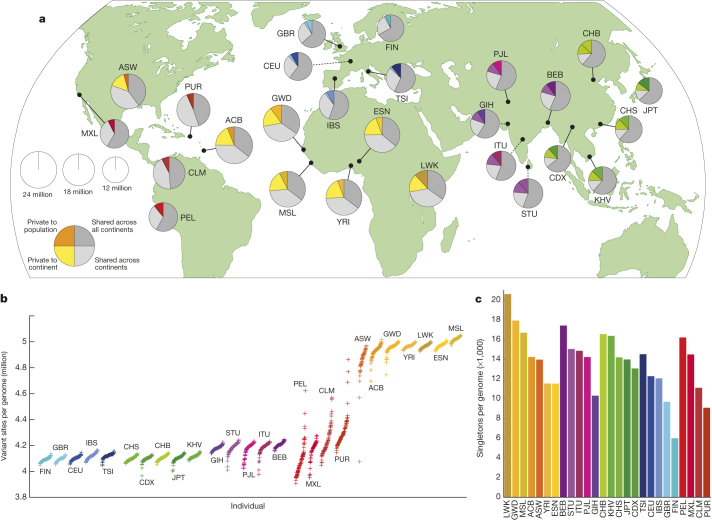
In this final phase, individuals were sampled from 26 populations in Africa (AFR), East Asia (EAS), Europe (EUR), South Asia (SAS), and the Americas (AMR) (Fig. 1a; see Supplementary Table 1 for population descriptions and abbreviations). All individuals were sequenced using both whole-genome sequencing (mean depth = 7.4×) and targeted exome sequencing (mean depth = 65.7×). In addition, individuals and available first-degree relatives (generally, adult offspring) were genotyped using high-density SNP microarrays. This provided a cost-effective means to discover genetic variants and estimate individual genotypes and haplotypes1,2.
Figure 1. Population sampling.
a, Polymorphic variants within sampled populations. The area of each pie is proportional to the number of polymorphisms within a population. Pies are divided into four slices, representing variants private to a population (darker colour unique to population), private to a continental area (lighter colour shared across continental group), shared across continental areas (light grey), and shared across all continents (dark grey). Dashed lines indicate populations sampled outside of their ancestral continental region. b, The number of variant sites per genome. c, The average number of singletons per genome.
Data set overview
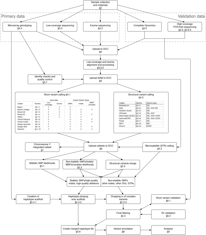
In contrast to earlier phases of the project, we expanded analysis beyond bi-allelic events to include multi-allelic SNPs, indels, and a diverse set of structural variants (SVs). An overview of the sample collection, data generation, data processing, and analysis is given in Extended Data Fig. 1. Variant discovery used an ensemble of 24 sequence analysis tools (Supplementary Table 2), and machine-learning classifiers to separate high-quality variants from potential false positives, balancing sensitivity and specificity. Construction of haplotypes started with estimation of long-range phased haplotypes using array genotypes for project participants and, where available, their first degree relatives; continued with the addition of high confidence bi-allelic variants that were analysed jointly to improve these haplotypes; and concluded with the placement of multi-allelic and structural variants onto the haplotype scaffold one at a time (Box 1). Overall, we discovered, genotyped, and phased 88 million variant sites (Supplementary Table 3). The project has now contributed or validated 80 million of the 100 million variants in the public dbSNP catalogue (version 141 includes 40 million SNPs and indels newly contributed by this analysis). These novel variants especially enhance our catalogue of genetic variation within South Asian (which account for 24% of novel variants) and African populations (28% of novel variants).
Extended Data Figure 1. Summary of the callset generation pipeline.
Boxes indicate steps in the process and numbers indicate the corresponding section(s) within the Supplementary Information.
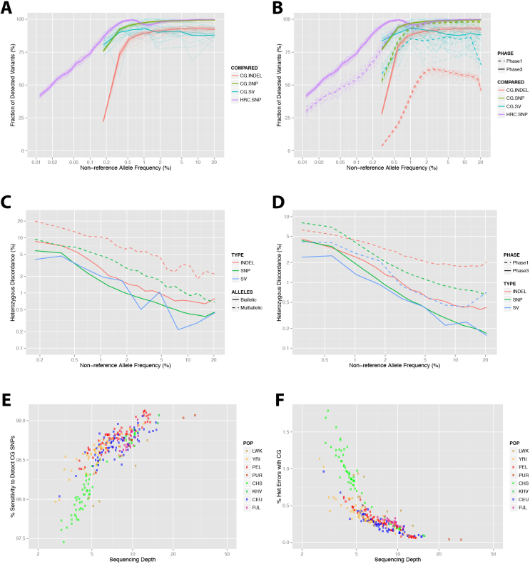
To control the false discovery rate (FDR) of SNPs and indels at <5%, a variant quality score threshold was defined using high depth (>30×) PCR-free sequence data generated for one individual per population. For structural variants, additional orthogonal methods were used for confirmation, including microarrays and long-read sequencing, resulting in FDR < 5% for deletions, duplications, multi-allelic copy-number variants, Alu and L1 insertions, and <20% for inversions, SVA (SINE/VNTR/Alu) composite retrotransposon insertions and NUMTs8 (nuclear mitochondrial DNA variants). To evaluate variant discovery power and genotyping accuracy, we also generated deep Complete Genomics data (mean depth = 47×) for 427 individuals (129 mother–father–child trios, 12 parent–child duos, and 16 unrelateds). We estimate the power to detect SNPs and indels to be >95% and >80%, respectively, for variants with sample frequency of at least 0.5%, rising to >99% and >85% for frequencies >1% (Extended Data Fig. 2). At lower frequencies, comparison with >60,000 European haplotypes from the Haplotype Reference Consortium9 suggests 75% power to detect SNPs with frequency of 0.1%. Furthermore, we estimate heterozygous genotype accuracy at 99.4% for SNPs and 99.0% for indels (Supplementary Table 4), a threefold reduction in error rates compared to our previous release2, resulting from the larger sample size, improvements in sequence data accuracy, and genotype calling and phasing algorithms.
Extended Data Figure 2. Power of discovery and heterozygote genotype discordance.
a, The power of discovery within the main data set for SNPs and indels identified within an overlapping sample of 284 genomes sequenced to high coverage by Complete Genomics (CG), and against a panel of >60,000 haplotypes constructed by the Haplotype Reference Consortium (HRC)9. To provide a measure of uncertainty, one curve is plotted for each chromosome. b, Improved power of discovery in phase 3 compared to phase 1, as assessed in a sample of 170 Complete Genomics genomes that are included in both phase 1 and phase 3. c, Heterozygote discordance in phase 3 for SNPs, indels, and SVs compared to 284 Complete Genomics genomes. d, Heterozygote discordance for phase 3 compared to phase 1 within the intersecting sample. e, Sensitivity to detect Complete Genomics SNPs as a function of sequencing depth. f, Heterozygote genotype discordance as a function of sequencing depth, as compared to Complete Genomics data.
Box 1: Building a haplotype scaffold.
To construct high quality haplotypes that integrate multiple variant types, we adopted a staged approach37. (1) A high-quality ‘haplotype scaffold’ was constructed using statistical methods applied to SNP microarray genotypes (black circles) and, where available, genotypes for first degree relatives (available for ∼52% of samples; Supplementary Table 11)38. (2a) Variant sites were identified using a combination of bioinformatic tools and pipelines to define a set of high-confidence bi-allelic variants, including both SNPs and indels (white triangles), which were jointly imputed onto the haplotype scaffold. (2b) Multi-allelic SNPs, indels, and complex variants (represented by yellow shapes, or variation in copy number) were placed onto the haplotype scaffold one at a time, exploiting the local linkage disequilibrium information but leaving haplotypes for other variants undisturbed39. (3) The biallelic and multi-allelic haplotypes were merged into a single haplotype representation. This multi-stage approach allows the long-range structure of the haplotype scaffold to be maintained while including more complex types of variation. Comparison to haplotypes constructed from fosmids suggests the average distance between phasing errors is ∼1,062 kb, with typical phasing errors stretching ∼37 kb (Supplementary Table 12).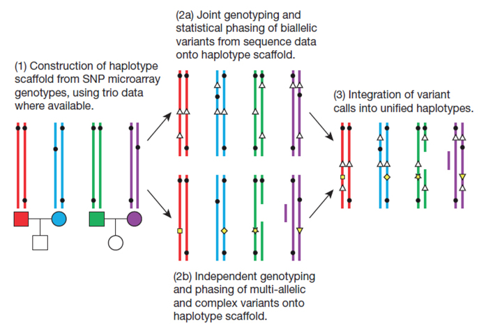
A typical genome
We find that a typical genome differs from the reference human genome at 4.1 million to 5.0 million sites (Fig. 1b and Table 1). Although >99.9% of variants consist of SNPs and short indels, structural variants affect more bases: the typical genome contains an estimated 2,100 to 2,500 structural variants (∼1,000 large deletions, ∼160 copy-number variants, ∼915 Alu insertions, ∼128 L1 insertions, ∼51 SVA insertions, ∼4 NUMTs, and ∼10 inversions), affecting ∼20 million bases of sequence.
Table 1.
Median autosomal variant sites per genome
| AFR | AMR | EAS | EUR | SAS | ||||||
|---|---|---|---|---|---|---|---|---|---|---|
| Samples | 661 | 347 | 504 | 503 | 489 | |||||
| Mean coverage | 8.2 | 7.6 | 7.7 | 7.4 | 8.0 | |||||
| Var. sites | Singletons | Var. sites | Singletons | Var. sites | Singletons | Var. sites | Singletons | Var. sites | Singletons | |
| SNPs | 4.31M | 14.5k | 3.64M | 12.0k | 3.55M | 14.8k | 3.53M | 11.4k | 3.60M | 14.4k |
| Indels | 625k | - | 557k | - | 546k | - | 546k | - | 556k | - |
| Large deletions | 1.1k | 5 | 949 | 5 | 940 | 7 | 939 | 5 | 947 | 5 |
| CNVs | 170 | 1 | 153 | 1 | 158 | 1 | 157 | 1 | 165 | 1 |
| MEI (Alu) | 1.03k | 0 | 845 | 0 | 899 | 1 | 919 | 0 | 889 | 0 |
| MEI (L1) | 138 | 0 | 118 | 0 | 130 | 0 | 123 | 0 | 123 | 0 |
| MEI (SVA) | 52 | 0 | 44 | 0 | 56 | 0 | 53 | 0 | 44 | 0 |
| MEI (MT) | 5 | 0 | 5 | 0 | 4 | 0 | 4 | 0 | 4 | 0 |
| Inversions | 12 | 0 | 9 | 0 | 10 | 0 | 9 | 0 | 11 | 0 |
| Nonsynon | 12.2k | 139 | 10.4k | 121 | 10.2k | 144 | 10.2k | 116 | 10.3k | 144 |
| Synon | 13.8k | 78 | 11.4k | 67 | 11.2k | 79 | 11.2k | 59 | 11.4k | 78 |
| Intron | 2.06M | 7.33k | 1.72M | 6.12k | 1.68M | 7.39k | 1.68M | 5.68k | 1.72M | 7.20k |
| UTR | 37.2k | 168 | 30.8k | 136 | 30.0k | 169 | 30.0k | 129 | 30.7k | 168 |
| Promoter | 102k | 430 | 84.3k | 332 | 81.6k | 425 | 82.2k | 336 | 84.0k | 430 |
| Insulator | 70.9k | 248 | 59.0k | 199 | 57.7k | 252 | 57.7k | 189 | 59.1k | 243 |
| Enhancer | 354k | 1.32k | 295k | 1.05k | 289k | 1.34k | 288k | 1.02k | 295k | 1.31k |
| TFBSs | 927 | 4 | 759 | 3 | 748 | 4 | 749 | 3 | 765 | 3 |
| Filtered LoF | 182 | 4 | 152 | 3 | 153 | 4 | 149 | 3 | 151 | 3 |
| HGMD-DM | 20 | 0 | 18 | 0 | 16 | 1 | 18 | 2 | 16 | 0 |
| GWAS | 2.00k | 0 | 2.07k | 0 | 1.99k | 0 | 2.08k | 0 | 2.06k | 0 |
| ClinVar | 28 | 0 | 30 | 1 | 24 | 0 | 29 | 1 | 27 | 1 |
The total number of observed non-reference sites differs greatly among populations (Fig. 1b). Individuals from African ancestry populations harbour the greatest numbers of variant sites, as predicted by the out-of-Africa model of human origins. Individuals from recently admixed populations show great variability in the number of variants, roughly proportional to the degree of recent African ancestry in their genomes.
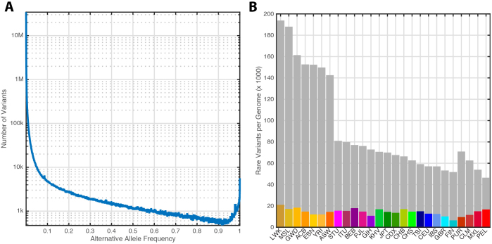
The majority of variants in the data set are rare: ∼64 million autosomal variants have a frequency <0.5%, ∼12 million have a frequency between 0.5% and 5%, and only ∼8 million have a frequency >5% (Extended Data Fig. 3a). Nevertheless, the majority of variants observed in a single genome are common: just 40,000 to 200,000 of the variants in a typical genome (1–4%) have a frequency <0.5% (Fig. 1c and Extended Data Fig. 3b). As such, we estimate that improved rare variant discovery by deep sequencing our entire sample would at least double the total number of variants in our sample but increase the number of variants in a typical genome by only ∼20,000 to 60,000.
Extended Data Figure 3. Variant counts.
a, The number of variants within the phase 3 sample as a function of alternative allele frequency. b, The average number of detected variants per genome with whole-sample allele frequencies <0.5% (grey bars), with the average number of singletons indicated by colours.
Putatively functional variation
When we restricted analyses to the variants most likely to affect gene function, we found a typical genome contained 149–182 sites with protein truncating variants, 10,000 to 12,000 sites with peptide-sequence-altering variants, and 459,000 to 565,000 variant sites overlapping known regulatory regions (untranslated regions (UTRs), promoters, insulators, enhancers, and transcription factor binding sites). African genomes were consistently at the high end of these ranges. The number of alleles associated with a disease or phenotype in each genome did not follow this pattern of increased diversity in Africa (Extended Data Fig. 4): we observed ∼2,000 variants per genome associated with complex traits through genome-wide association studies (GWAS) and 24–30 variants per genome implicated in rare disease through ClinVar; with European ancestry genomes at the high-end of these counts. The magnitude of this difference is unlikely to be explained by demography10,11, but instead reflects the ethnic bias of current genetic studies. We expect that improved characterization of the clinical and phenotypic consequences of non-European alleles will enable better interpretation of genomes from all individuals and populations.
Extended Data Figure 4. The standardized number of variant sites per genome, partitioned by population and variant category.
For each category, _z_-scores were calculated by subtracting the mean number of sites per genome (calculated across the whole sample), and dividing by the standard deviation. From left: sites with a derived allele, synonymous sites with a derived allele, nonsynonymous sites with a derived allele, sites with a loss-of-function allele, sites with a HGMD disease mutation allele, sites with a ClinVar pathogenic variant, and sites carrying a GWAS risk allele.
Sharing of genetic variants among populations
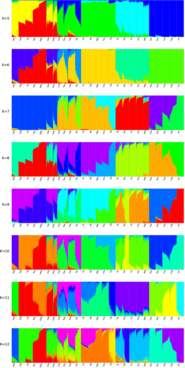
Systematic analysis of the patterns in which genetic variants are shared among individuals and populations provides detailed accounts of population history. Although most common variants are shared across the world, rarer variants are typically restricted to closely related populations (Fig. 1a); 86% of variants were restricted to a single continental group. Using a maximum likelihood approach12, we estimated the proportion of each genome derived from several putative ‘ancestral populations’ (Fig. 2a and Extended Data Fig. 5). This analysis separates continental groups, highlights their internal substructure, and reveals genetic similarities between related populations. For example, east–west clines are visible in Africa and East Asia, a north–south cline is visible in Europe, and European, African, and Native-American admixture is visible in genomes sampled in the Americas.
Figure 2. Population structure and demography.
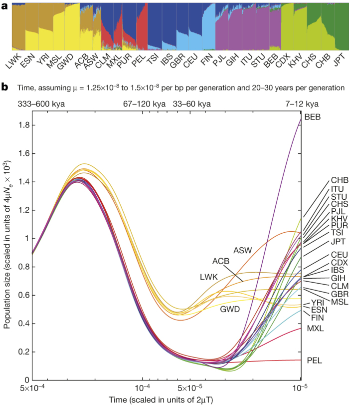
a, Population structure inferred using a maximum likelihood approach with 8 clusters. b, Changes to effective population sizes over time, inferred using PSMC. Lines represent the within-population median PSMC estimate, smoothed by fitting a cubic spline passing through bin midpoints.
Extended Data Figure 5. Population structure as inferred using the admixture program for K = 5 to 12.
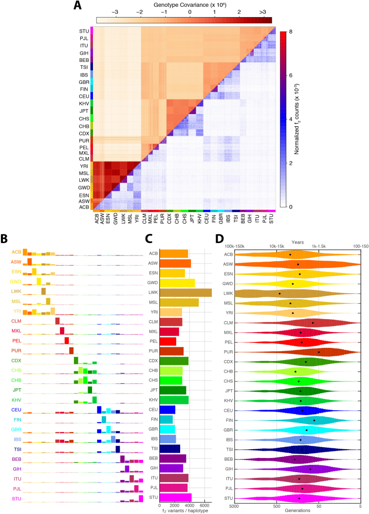
To characterize more recent patterns of shared ancestry, we first focused on variants observed on just two chromosomes (sample frequency of 0.04%), the rarest shared variants within our sample, and known as _f_2 variants2. As expected, these variants are typically geographically restricted and much more likely to be shared between individuals in the same population or continental group, or between populations with known recent admixture (Extended Data Fig. 6a, b). Analysis of shared haplotype lengths around _f_2 variants suggests a median common ancestor ∼296 generations ago (7,410 to 8,892 years ago; Extended Data Fig. 6c, d), although those confined within a population tend to be younger, with a shared common ancestor ∼143 generations ago (3,570 to 4,284 years ago)13.
Extended Data Figure 6. Allelic sharing.
a, Genotype covariance (above diagonal) and sharing of _f_2 variants (below diagonal) between pairs of individuals. b, Quantification of average _f_2 sharing between populations. Each row represents the distribution of _f_2 variants shared between individuals from the population indicated on the left to individuals from each of the sampled populations. c, The average number of _f_2 variants per haploid genome. d, The inferred age of _f_2 variants, as estimated from shared haplotype lengths, with black dots indicating the median value.
Insights about demography
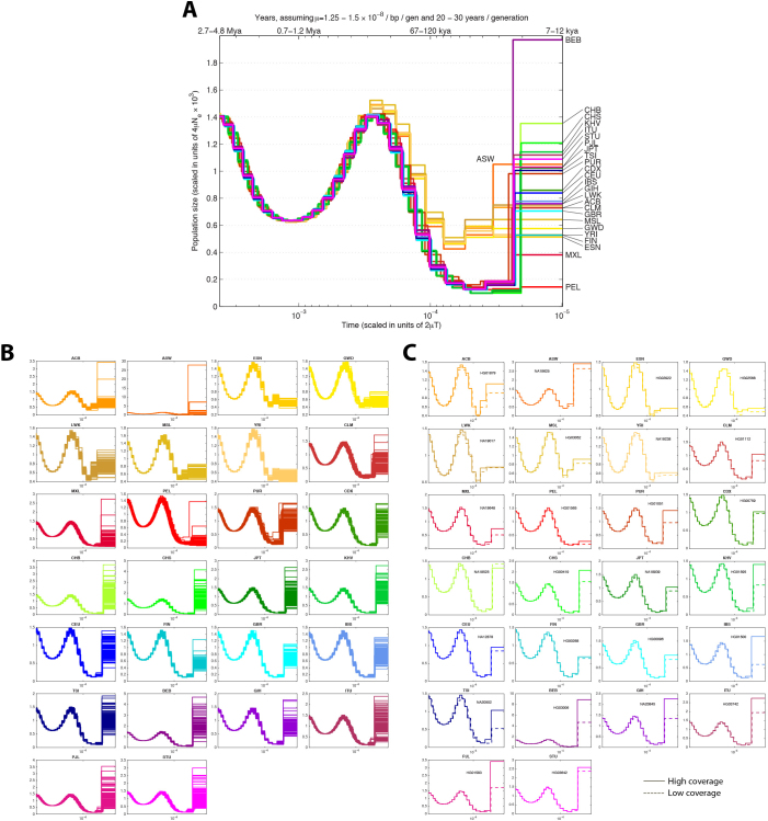
Modelling the distribution of variation within and between genomes can provide insights about the history and demography of our ancestor populations14. We used the pairwise sequentially Markovian coalescent (PSMC)14 method to characterize the effective population size (N e) of the ancestral populations (Fig. 2b and Extended Data Fig. 7). Our results show a shared demographic history for all humans beyond ∼150,000 to 200,000 years ago. Further, they show that European, Asian and American populations shared strong and sustained bottlenecks, all with N e < 1,500, between 15,000 to 20,000 years ago. In contrast, the bottleneck experienced by African populations during the same time period appears less severe, with _N_ _e_ > 4,250. These bottlenecks were followed by extremely rapid inferred population growth in non-African populations, with notable exceptions including the PEL, MXL and FIN.
Extended Data Figure 7. Unsmoothed PSMC curves.
a, The median PSMC curve for each population. b, PSMC curves estimated separately for all individuals within the 1000 Genomes sample. c, Unsmoothed PSMC curves comparing estimates from the low coverage data (dashed lines) to those obtained from high coverage PCR-free data (solid lines). Notable differences are confined to very recent time intervals, where the additional rare variants identified by deep sequencing suggest larger population sizes.
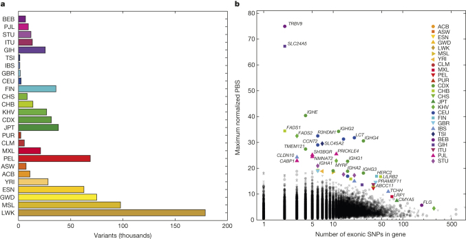
Due to the shared ancestry of all humans, only a modest number of variants show large frequency differences among populations. We observed 762,000 variants that are rare (defined as having frequency <0.5%) within the global sample but much more common (>5% frequency) in at least one population (Fig. 3a). Several populations have relatively large numbers of these variants, and these are typically genetically or geographically distinct within their continental group (LWK in Africa, PEL in the Americas, JPT in East Asia, FIN in Europe, and GIH in South Asia; see Supplementary Table 5). Drifted variants within such populations may reveal phenotypic associations that would be hard to identify in much larger global samples15.
Figure 3. Population differentiation.
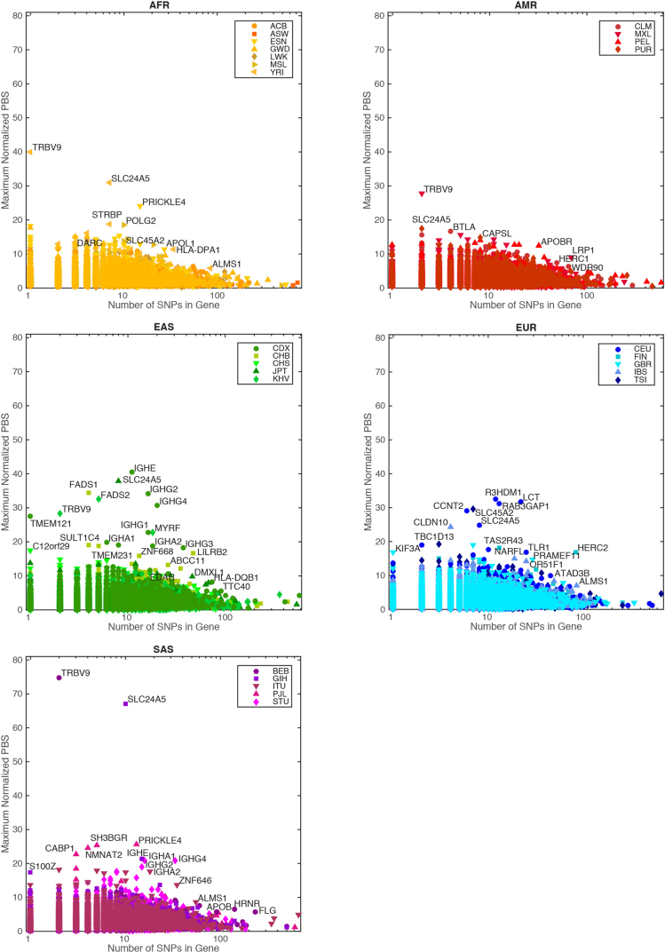
a, Variants found to be rare (<0.5%) within the global sample, but common (>5%) within a population. b, Genes showing strong differentiation between pairs of closely related populations. The vertical axis gives the maximum obtained value of the _F_ST-based population branch statistic (PBS), with selected genes coloured to indicate the population in which the maximum value was achieved.
Analysis of the small set of variants with large frequency differences between closely related populations can identify targets of recent, localized adaptation. We used the _F_ST-based population branch statistic (PBS)16 to identify genes with strong differentiation between pairs of populations in the same continental group (Fig. 3b). This approach reveals a number of previously identified selection signals (such as SLC24A5 associated with skin pigmentation17, HERC2 associated with eye colour18, LCT associated with lactose tolerance, and the FADS cluster that may be associated with dietary fat sources19). Several potentially novel selection signals are also highlighted (such as TRBV9, which appears particularly differentiated in South Asia, PRICKLE4, differentiated in African and South Asian populations, and a number of genes in the immunoglobulin cluster, differentiated in East Asian populations; Extended Data Fig. 8), although at least some of these signals may result from somatic rearrangements (for example, via V(D)J recombination) and differences in cell type composition among the sequenced samples. Nonetheless, the relatively small number of genes showing strong differentiation between closely related populations highlights the rarity of strong selective sweeps in recent human evolution20.
Extended Data Figure 8. Genes showing very strong patterns of differentiation between pairs of closely related populations within each continental group.
Within each continental group, the maximum PBS statistic was selected from all pairwise population comparisons within the continental group against all possible out-of-continent populations. Note the x axis shows the number of polymorphic sites within the maximal comparison.
Sharing of haplotypes and imputation
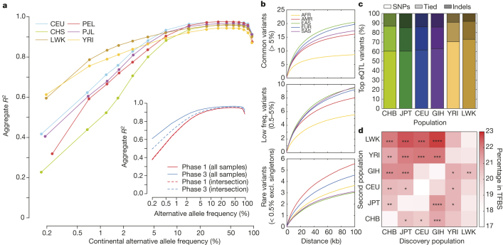
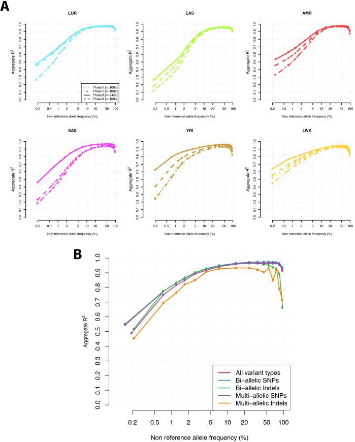
The sharing of haplotypes among individuals is widely used for imputation in GWAS, a primary use of 1000 Genomes data. To assess imputation based on the phase 3 data set, we used Complete Genomics data for 9 or 10 individuals from each of 6 populations (CEU, CHS, LWK, PEL, PJL, and YRI). After excluding these individuals from the reference panel, we imputed genotypes across the genome using sites on a typical one million SNP microarray. The squared correlation between imputed and experimental genotypes was >95% for common variants in each population, decreasing gradually with minor allele frequency (Fig. 4a). Compared to phase 1, rare variation imputation improved considerably, particularly for newly sampled populations (for example, PEL and PJL, Extended Data Fig. 9a). Improvements in imputations restricted to overlapping samples suggest approximately equal contributions from greater genotype and sequence quality and from increased sample size (Fig. 4a, inset). Imputation accuracy is now similar for bi-allelic SNPs, bi-allelic indels, multi-allelic SNPs, and sites where indels and SNPs overlap, but slightly reduced for multi-allelic indels, which typically map to regions of low-complexity sequence and are much harder to genotype and phase (Extended Data Fig. 9b). Although imputation of rare variation remains challenging, it appears to be most accurate in African ancestry populations, where greater genetic diversity results in a larger number of haplotypes and improves the chances that a rare variant is tagged by a characteristic haplotype.
Figure 4. Imputation and eQTL discovery.
a, Imputation accuracy as a function of allele frequency for six populations. The insert compares imputation accuracy between phase 3 and phase 1, using all samples (solid lines) and intersecting samples (dashed lines). b, The average number of tagging variants (_r_2 > 0.8) as a function of physical distance for common (top), low frequency (middle), and rare (bottom) variants. c, The proportion of top eQTL variants that are SNPs and indels, as discovered in 69 samples from each population. d, The percentage of eQTLs in TFBS, having performed discovery in the first population, and fine mapped by including an additional 69 samples from a second population (*P < 0.01, **P < 0.001, ***P < 0.0001, McNemar’s test). The diagonal represents the percentage of eQTLs in TFBS using the original discovery sample.
Extended Data Figure 9. Performance of imputation.
a, Performance of imputation in 6 populations using a subset of phase 3 as a reference panel (n = 2,445), phase 1 (n = 1,065), and the corresponding data within intersecting samples from both phases (n = 1,006). b, Performance of imputation from phase 3 by variant class.
Resolution of genetic association studies
To evaluate the impact of our new reference panel on GWAS, we re-analysed a previous study of age-related macular degeneration (AMD) totalling 2,157 cases and 1,150 controls21. We imputed 17.0 million genetic variants with estimated _R_2 > 0.3, compared to 14.1 million variants using phase 1, and only 2.4 million SNPs using HapMap2. Compared to phase 1, the number of imputed common and intermediate frequency variants increased by 7%, whereas the number of rare variants increased by >50%, and the number of indels increased by 70% (Supplementary Table 6). We permuted case-control labels to estimate a genome-wide significance threshold of P < ∼1.5 × 10⁻⁸, which corresponds to ∼3 million independent variants and is more stringent than the traditional threshold of 5 × 10⁻⁸ (Supplementary Table 7). In practice, significance thresholds must balance false positives and false negatives22,23,24. We recommend that thresholds aiming for strict control of false positives should be determined using permutations. We expect thresholds to become more stringent when larger sample sizes are sequenced, when diverse samples are studied, or when genotyping and imputation is replaced with direct sequencing. After imputation, five independent signals in four previously reported AMD loci25,26,27,28 reached genome-wide significance (Supplementary Table 8). When we examined each of these to define a set of potentially causal variants using a Bayesian Credible set approach29, lists of potentially functional variants were ∼4× larger than in HapMap2-based analysis and 7% larger than in analyses based on phase 1 (Supplementary Table 9). In the ARMS2/HTRA1 locus, the most strongly associated variant was now a structural variant (estimated imputation _R_2 = 0.89) that previously could not be imputed, consistent with some functional studies30. Deep catalogues of potentially functional variants will help ensure that downstream functional analyses include the true candidate variants, and will aid analyses that integrate complex disease associations with functional genomic elements31.
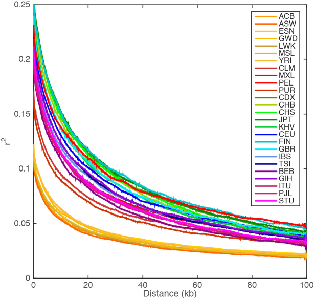
The performance of imputation and GWAS studies depends on the local distribution of linkage disequilibrium (LD) between nearby variants. Controlling for sample size, the decay of LD as a function of physical distance is fastest in African populations and slowest in East Asian populations (Extended Data Fig. 10). To evaluate how these differences influence the resolution of genetic association studies and, in particular, their ability to identify a narrow set of candidate functional variants, we evaluated the number of tagging variants (_r_2 > 0.8) for a typical variant in each population. We find that each common variant typically has over 15–20 tagging variants in non-African populations, but only about 8 in African populations (Fig. 4b). At lower frequencies, we find 3–6 tagging variants with 100 kb of variants with frequency <0.5%, and differences in the number of tagging variants between continental groups are less marked.
Extended Data Figure 10. Decay of linkage disequilibrium as a function of physical distance.
Linkage disequilibrium was calculated around 10,000 randomly selected polymorphic sites in each population, having first thinned each population down to the same sample size (61 individuals). The plotted line represents a 5 kb moving average.
Among variants in the GWAS catalogue (which have an average frequency of 26.6% in project haplotypes), the number of proxies averages 14.4 in African populations and 30.3–44.4 in other continental groupings (Supplementary Table 10). The potential value of multi-population fine-mapping is illustrated by the observation that the number of proxies shared across all populations is only 8.2 and, furthermore, that 34.9% of GWAS catalogue variants have no proxy shared across all continental groupings.
To further assess prospects for fine-mapping genetic association signals, we performed expression quantitative trait loci (eQTL) discovery at 17,667 genes in 69 samples from each of 6 populations (CEU, CHB, GIH, JPT, LWK, and YRI)32. We identified eQTLs for 3,285 genes at 5% FDR (average 1,265 genes per population). Overall, a typical eQTL signal comprised 67 associated variants, including an indel as one of the top associated variants 26–40% of the time (Fig. 4c). Within each discovery population, 17.5–19.5% of top eQTL variants overlapped annotated transcription factor binding sites (TFBSs), consistent with the idea that a substantial fraction of eQTL polymorphisms are TFBS polymorphisms. Using a meta-analysis approach to combine pairs of populations, the proportion of top eQTL variants overlapping TFBSs increased to 19.2–21.6% (Fig. 4d), consistent with improved localization. Including an African population provided the greatest reduction in the count of associated variants and the greatest increase in overlap between top variants and TFBSs.
Discussion
Over the course of the 1000 Genomes Project there have been substantial advances in sequence data generation, archiving and analysis. Primary sequence data production improved with increased read length and depth, reduced per-base errors, and the introduction of paired-end sequencing. Sequence analysis methods improved with the development of strategies for identifying and filtering poor-quality data, for more accurate mapping of sequence reads (particularly in repetitive regions), for exchanging data between analysis tools and enabling ensemble analyses, and for capturing more diverse types of variants. Importantly, each release has examined larger numbers of individuals, aiding population-based analyses that identify and leverage shared haplotypes during genotyping. Whereas our first analyses produced high-confidence short-variant calls for 80–85% of the reference genome1, our newest analyses reach ∼96% of the genome using the same metrics, although our ability to accurately capture structural variation remains more limited33. In addition, the evolution of sequencing, analysis and filtering strategies means that our results are not a simple superset of previous analysis. Although the number of characterized variants has more than doubled relative to phase 1, ∼2.3 million previously described variants are not included in the current analysis; most missing variants were rare or marked as low quality: 1.6 million had frequency <0.5% and may be missing from our current read set, while the remainder were removed by our filtering processes.
These same technical advances are enabling the application of whole genome sequencing to a variety of medically important samples. Some of these studies already exceed the 1000 Genomes Project in size34,35,36, but the results described here remain a prime resource for studies of genetic variation for several reasons. First, the 1000 Genomes Project samples provide a broad representation of human genetic variation—in contrast to the bulk of complex disease studies in humans, which primarily study European ancestry samples and which, as we show, fail to capture functionally important variation in other populations. Second, the project analyses incorporate multiple analysis strategies, callsets and variant types. Although such ensemble analyses are cumbersome, they provide a benchmark for what can be achieved and a yardstick against which more practical analysis strategies can be evaluated. Third, project samples and data resulting from them can be shared broadly, enabling sequencing strategies and analysis methods to be compared easily on a benchmark set of samples. Because of the wide availability of the data and samples, these samples have been and will continue to be used for studying many molecular phenotypes. Thus, we predict that the samples will accumulate many types of data that will allow connections to be drawn between variants and both molecular and disease phenotypes.
Supplementary information
Acknowledgements
We thank the many people who were generous with contributing their samples to the project: the African Caribbean in Barbados; Bengali in Bangladesh; British in England and Scotland; Chinese Dai in Xishuangbanna, China; Colombians in Medellin, Colombia; Esan in Nigeria; Finnish in Finland; Gambian in Western Division – Mandinka; Gujarati Indians in Houston, Texas, USA; Han Chinese in Beijing, China; Iberian populations in Spain; Indian Telugu in the UK; Japanese in Tokyo, Japan; Kinh in Ho Chi Minh City, Vietnam; Luhya in Webuye, Kenya; Mende in Sierra Leone; people with African ancestry in the southwest USA; people with Mexican ancestry in Los Angeles, California, USA; Peruvians in Lima, Peru; Puerto Ricans in Puerto Rico; Punjabi in Lahore, Pakistan; southern Han Chinese; Sri Lankan Tamil in the UK; Toscani in Italia; Utah residents (CEPH) with northern and western European ancestry; and Yoruba in Ibadan, Nigeria. Many thanks to the people who contributed to this project: P. Maul, T. Maul, and C. Foster; Z. Chong, X. Fan, W. Zhou, and T. Chen; N. Sengamalay, S. Ott, L. Sadzewicz, J. Liu, and L. Tallon; L. Merson; O. Folarin, D. Asogun, O. Ikpwonmosa, E. Philomena, G. Akpede, S. Okhobgenin, and O. Omoniwa; the staff of the Institute of Lassa Fever Research and Control (ILFRC), Irrua Specialist Teaching Hospital, Irrua, Edo State, Nigeria; A. Schlattl and T. Zichner; S. Lewis, E. Appelbaum, and L. Fulton; A. Yurovsky and I. Padioleau; N. Kaelin and F. Laplace; E. Drury and H. Arbery; A. Naranjo, M. Victoria Parra, and C. Duque; S. Dökel, B. Lenz, and S. Schrinner; S. Bumpstead; and C. Fletcher-Hoppe. Funding for this work was from the Wellcome Trust Core Award 090532/Z/09/Z and Senior Investigator Award 095552/Z/11/Z (P.D.), and grants WT098051 (R.D.), WT095908 and WT109497 (P.F.), WT086084/Z/08/Z and WT100956/Z/13/Z (G.M.), WT097307 (W.K.), WT0855322/Z/08/Z (R.L.), WT090770/Z/09/Z (D.K.), the Wellcome Trust Major Overseas program in Vietnam grant 089276/Z.09/Z (S.D.), the Medical Research Council UK grant G0801823 (J.L.M.), the UK Biotechnology and Biological Sciences Research Council grants BB/I02593X/1 (G.M.) and BB/I021213/1 (A.R.L.), the British Heart Foundation (C.A.A.), the Monument Trust (J.H.), the European Molecular Biology Laboratory (P.F.), the European Research Council grant 617306 (J.L.M.), the Chinese 863 Program 2012AA02A201, the National Basic Research program of China 973 program no. 2011CB809201, 2011CB809202 and 2011CB809203, Natural Science Foundation of China 31161130357, the Shenzhen Municipal Government of China grant ZYC201105170397A (J.W.), the Canadian Institutes of Health Research Operating grant 136855 and Canada Research Chair (S.G.), Banting Postdoctoral Fellowship from the Canadian Institutes of Health Research (M.K.D.), a Le Fonds de Recherche du Québec-Santé (FRQS) research fellowship (A.H.), Genome Quebec (P.A.), the Ontario Ministry of Research and Innovation – Ontario Institute for Cancer Research Investigator Award (P.A., J.S.), the Quebec Ministry of Economic Development, Innovation, and Exports grant PSR-SIIRI-195 (P.A.), the German Federal Ministry of Education and Research (BMBF) grants 0315428A and 01GS08201 (R.H.), the Max Planck Society (H.L., G.M., R.S.), BMBF-EPITREAT grant 0316190A (R.H., M.L.), the German Research Foundation (Deutsche Forschungsgemeinschaft) Emmy Noether Grant KO4037/1-1 (J.O.K.), the Beatriu de Pinos Program grants 2006 BP-A 10144 and 2009 BP-B 00274 (M.V.), the Spanish National Institute for Health Research grant PRB2 IPT13/0001-ISCIII-SGEFI/FEDER (A.O.), Ewha Womans University (C.L.), the Japan Society for the Promotion of Science Fellowship number PE13075 (N.P.), the Louis Jeantet Foundation (E.T.D.), the Marie Curie Actions Career Integration grant 303772 (C.A.), the Swiss National Science Foundation 31003A_130342 and NCCR “Frontiers in Genetics” (E.T.D.), the University of Geneva (E.T.D., T.L., G.M.), the US National Institutes of Health National Center for Biotechnology Information (S.S.) and grants U54HG3067 (E.S.L.), U54HG3273 and U01HG5211 (R.A.G.), U54HG3079 (R.K.W., E.R.M.), R01HG2898 (S.E.D.), R01HG2385 (E.E.E.), RC2HG5552 and U01HG6513 (G.T.M., G.R.A.), U01HG5214 (A.C.), U01HG5715 (C.D.B.), U01HG5718 (M.G.), U01HG5728 (Y.X.F.), U41HG7635 (R.K.W., E.E.E., P.H.S.), U41HG7497 (C.L., M.A.B., K.C., L.D., E.E.E., M.G., J.O.K., G.T.M., S.A.M., R.E.M., J.L.S., K.Y.), R01HG4960 and R01HG5701 (B.L.B.), R01HG5214 (G.A.), R01HG6855 (S.M.), R01HG7068 (R.E.M.), R01HG7644 (R.D.H.), DP2OD6514 (P.S.), DP5OD9154 (J.K.), R01CA166661 (S.E.D.), R01CA172652 (K.C.), P01GM99568 (S.R.B.), R01GM59290 (L.B.J., M.A.B.), R01GM104390 (L.B.J., M.Y.Y.), T32GM7790 (C.D.B., A.R.M.), P01GM99568 (S.R.B.), R01HL87699 and R01HL104608 (K.C.B.), T32HL94284 (J.L.R.F.), and contracts HHSN268201100040C (A.M.R.) and HHSN272201000025C (P.S.), Harvard Medical School Eleanor and Miles Shore Fellowship (K.L.), Lundbeck Foundation Grant R170-2014-1039 (K.L.), NIJ Grant 2014-DN-BX-K089 (Y.E.), the Mary Beryl Patch Turnbull Scholar Program (K.C.B.), NSF Graduate Research Fellowship DGE-1147470 (G.D.P.), the Simons Foundation SFARI award SF51 (M.W.), and a Sloan Foundation Fellowship (R.D.H.). E.E.E. is an investigator of the Howard Hughes Medical Institute.
Extended data figures and tables
Related audio
Adam Levy investigates the huge progress made in the 25 years since Human Genome Project began.
PowerPoint slides
Author Contributions
Details of author contributions can be found in the author list.
Competing interests
D.M.A. is affiliated with Vertex Pharmaceuticals, E.A. is on the speaker’s bureau for Illumina, P.A. is an advisor to Illumina and Ancestry.com, D.R.B., B.B., M.B., R.K.C., A.C., M.E., S.H., S.K., L.M., J.P. and R.S. are affiliated with Illumina, J.K.B. is affiliated with Ancestry.com, A.C. is on the Science Advisory Board of Biogen Idec. and the scientific advisory board of Affymetrix, A.W.C. is affiliated with DNAnexus, D.C. is affiliated with Personalis, C.J.D., J.G., J.P.S., T.W., B.W., and Y.Z. are affiliated with Affymetrix, E.T.D. is an advisor for DNAnexus, F.M.D.L.V. is employed by Real Time Genomics, M.A.D. is affiliated with SynapDx, P.D. is a co-founder and director of Genomics, and a partner in Peptide Groove, R.D. is a founder of Congenica and a consultant for Dovetail, E.E.E. is on the scientific advisory board of DNAnexus, and is a consultant for Kunming University of Science and Technology as part of the 1000 China Talent Program, P.F. is a member of the scientific advisory board of Omicia, M.G. is an advisor to Bina and DNAnexus, F.C.L.H. is affiliated with ThermoFisher Scientific, N.H. is affiliated with Life Technologies, C.L. is a scientific advisor for BioNano Genomics, H.Y.K.L. is affiliated with Bina Technologies which is part of Roche Sequencing, E.R.M. holds shares in Life Technologies, and G.M. is a co-founder of Genomics and a partner in Peptide Groove.
Footnotes
(Participants are arranged by project role, then by institution alphabetically, and finally alphabetically within institutions except for Principal Investigators and Project Leaders, as indicated.)
Leena Peltonen: Deceased
Contributor Information
The 1000 Genomes Project Consortium:
Adam Auton, Gonçalo R. Abecasis, David M. Altshuler, (Co-Chair), Richard M. Durbin, (Co-Chair), Gonçalo R. Abecasis, David R. Bentley, Aravinda Chakravarti, Andrew G. Clark, Peter Donnelly, Evan E. Eichler, Paul Flicek, Stacey B. Gabriel, Richard A. Gibbs, Eric D. Green, Matthew E. Hurles, Bartha M. Knoppers, Jan O. Korbel, Eric S. Lander, Charles Lee, Hans Lehrach, Elaine R. Mardis, Gabor T. Marth, Gil A. McVean, Deborah A. Nickerson, Jeanette P. Schmidt, Stephen T. Sherry, Jun Wang, Richard K. Wilson, Aravinda Chakravarti, (Co-Chair), Bartha M. Knoppers, (Co-Chair), Gonçalo R. Abecasis, Kathleen C. Barnes, Christine Beiswanger, Esteban G. Burchard, Carlos D. Bustamante, Hongyu Cai, Hongzhi Cao, Richard M. Durbin, Norman P. Gerry, Neda Gharani, Richard A. Gibbs, Christopher R. Gignoux, Simon Gravel, Brenna Henn, Danielle Jones, Lynn Jorde, Jane S. Kaye, Alon Keinan, Alastair Kent, Angeliki Kerasidou, Yingrui Li, Rasika Mathias, Gil A. McVean, Andres Moreno-Estrada, Pilar N. Ossorio, Michael Parker, Alissa M. Resch, Charles N. Rotimi, Charmaine D. Royal, Karla Sandoval, Yeyang Su, Ralf Sudbrak, Zhongming Tian, Sarah Tishkoff, Lorraine H. Toji, Chris Tyler-Smith, Marc Via, Yuhong Wang, Huanming Yang, Ling Yang, Jiayong Zhu, Lisa D. Brooks, Adam L. Felsenfeld, Jean E. McEwen, Yekaterina Vaydylevich, Eric D. Green, Audrey Duncanson, Michael Dunn, Jeffery A. Schloss, Jun Wang, Huanming Yang, Adam Auton, Lisa D. Brooks, Richard M. Durbin, Erik P. Garrison, Hyun Min Kang, Jan O. Korbel, Jonathan L. Marchini, Shane McCarthy, Gil A. McVean, and Gonçalo R. Abecasis
References
- 1.The 1000 Genomes Project Consortium. A map of human genome variation from population-scale sequencing. Nature467, 1061–1073 (2010) [DOI] [PMC free article] [PubMed]
- 2.The 1000 Genomes Project Consortium. An integrated map of genetic variation from 1,092 human genomes. Nature491, 56–65 (2012) [DOI] [PMC free article] [PubMed]
- 3.Voight BF, et al. The metabochip, a custom genotyping array for genetic studies of metabolic, cardiovascular, and anthropometric traits. PLoS Genet. 2012;8:e1002793. doi: 10.1371/journal.pgen.1002793. [DOI] [PMC free article] [PubMed] [Google Scholar]
- 4.Trynka G, et al. Dense genotyping identifies and localizes multiple common and rare variant association signals in celiac disease. Nature Genet. 2011;43:1193–1201. doi: 10.1038/ng.998. [DOI] [PMC free article] [PubMed] [Google Scholar]
- 5.Howie B, Fuchsberger C, Stephens M, Marchini J, Abecasis GR. Fast and accurate genotype imputation in genome-wide association studies through pre-phasing. Nature Genet. 2012;44:955–959. doi: 10.1038/ng.2354. [DOI] [PMC free article] [PubMed] [Google Scholar]
- 6.Xue Y, et al. Deleterious- and disease-allele prevalence in healthy individuals: insights from current predictions, mutation databases, and population-scale resequencing. Am. J. Hum. Genet. 2012;91:1022–1032. doi: 10.1016/j.ajhg.2012.10.015. [DOI] [PMC free article] [PubMed] [Google Scholar]
- 7.Jung H, Bleazard T, Lee J, Hong D. Systematic investigation of cancer-associated somatic point mutations in SNP databases. Nature Biotechnol. 2013;31:787–789. doi: 10.1038/nbt.2681. [DOI] [PubMed] [Google Scholar]
- 8.Sudmant, P. H. et al. An integrated map of structural variation in 2,504 human genomes. _Nature_10.1038/nature15394 (this issue) [DOI] [PMC free article] [PubMed]
- 9.The Haplotype Reference Consortium (http://www.haplotype-reference-consortium.org/)
- 10.Simons YB, Turchin MC, Pritchard JK, Sella G. The deleterious mutation load is insensitive to recent population history. Nature Genet. 2014;46:220–224. doi: 10.1038/ng.2896. [DOI] [PMC free article] [PubMed] [Google Scholar]
- 11.Do R, et al. No evidence that selection has been less effective at removing deleterious mutations in Europeans than in Africans. Nature Genet. 2015;47:126–131. doi: 10.1038/ng.3186. [DOI] [PMC free article] [PubMed] [Google Scholar]
- 12.Alexander DH, Novembre J, Lange K. Fast model-based estimation of ancestry in unrelated individuals. Genome Res. 2009;19:1655–1664. doi: 10.1101/gr.094052.109. [DOI] [PMC free article] [PubMed] [Google Scholar]
- 13.Mathieson I, McVean G. Demography and the age of rare variants. PLoS Genet. 2014;10:e1004528. doi: 10.1371/journal.pgen.1004528. [DOI] [PMC free article] [PubMed] [Google Scholar]
- 14.Li H, Durbin R. Inference of human population history from individual whole-genome sequences. Nature. 2011;475:493–496. doi: 10.1038/nature10231. [DOI] [PMC free article] [PubMed] [Google Scholar]
- 15.Moltke I, et al. A common Greenlandic TBC1D4 variant confers muscle insulin resistance and type 2 diabetes. Nature. 2014;512:190–193. doi: 10.1038/nature13425. [DOI] [PubMed] [Google Scholar]
- 16.Yi X, et al. Sequencing of 50 human exomes reveals adaptation to high altitude. Science. 2010;329:75–78. doi: 10.1126/science.1190371. [DOI] [PMC free article] [PubMed] [Google Scholar]
- 17.Lamason RL, et al. SLC24A5, a putative cation exchanger, affects pigmentation in zebrafish and humans. Science. 2005;310:1782–1786. doi: 10.1126/science.1116238. [DOI] [PubMed] [Google Scholar]
- 18.Eiberg H, et al. Blue eye color in humans may be caused by a perfectly associated founder mutation in a regulatory element located within the HERC2 gene inhibiting OCA2 expression. Hum. Genet. 2008;123:177–187. doi: 10.1007/s00439-007-0460-x. [DOI] [PubMed] [Google Scholar]
- 19.Mathias RA, et al. Adaptive evolution of the FADS gene cluster within Africa. PLoS ONE. 2012;7:e44926. doi: 10.1371/journal.pone.0044926. [DOI] [PMC free article] [PubMed] [Google Scholar]
- 20.Hernandez RD, et al. Classic selective sweeps were rare in recent human evolution. Science. 2011;331:920–924. doi: 10.1126/science.1198878. [DOI] [PMC free article] [PubMed] [Google Scholar]
- 21.Chen W, et al. Genetic variants near TIMP3 and high-density lipoprotein-associated loci influence susceptibility to age-related macular degeneration. Proc. Natl Acad. Sci. USA. 2010;107:7401–7406. doi: 10.1073/pnas.0912702107. [DOI] [PMC free article] [PubMed] [Google Scholar]
- 22.Wakefield J. Bayes factors for genome-wide association studies: comparison with P-values. Genet. Epidemiol. 2009;33:79–86. doi: 10.1002/gepi.20359. [DOI] [PubMed] [Google Scholar]
- 23.Wakefield J. Commentary: genome-wide significance thresholds via Bayes factors. Int. J. Epidemiol. 2012;41:286–291. doi: 10.1093/ije/dyr241. [DOI] [PMC free article] [PubMed] [Google Scholar]
- 24.Sham PC, Purcell SM. Statistical power and significance testing in large-scale genetic studies. Nature Rev. Genet. 2014;15:335–346. doi: 10.1038/nrg3706. [DOI] [PubMed] [Google Scholar]
- 25.Gold B, et al. Variation in factor B (BF) and complement component 2 (C2) genes is associated with age-related macular degeneration. Nature Genet. 2006;38:458–462. doi: 10.1038/ng1750. [DOI] [PMC free article] [PubMed] [Google Scholar]
- 26.Klein RJ, et al. Complement factor H polymorphism in age-related macular degeneration. Science. 2005;308:385–389. doi: 10.1126/science.1109557. [DOI] [PMC free article] [PubMed] [Google Scholar]
- 27.Rivera A, et al. Hypothetical LOC387715 is a second major susceptibility gene for age-related macular degeneration, contributing independently of complement factor H to disease risk. Hum. Mol. Genet. 2005;14:3227–3236. doi: 10.1093/hmg/ddi353. [DOI] [PubMed] [Google Scholar]
- 28.Yates JR, et al. Complement C3 variant and the risk of age-related macular degeneration. N. Engl. J. Med. 2007;357:553–561. doi: 10.1056/NEJMoa072618. [DOI] [PubMed] [Google Scholar]
- 29.Maller JB, et al. Bayesian refinement of association signals for 14 loci in 3 common diseases. Nature Genet. 2012;44:1294–1301. doi: 10.1038/ng.2435. [DOI] [PMC free article] [PubMed] [Google Scholar]
- 30.Fritsche LG, et al. Age-related macular degeneration is associated with an unstable ARMS2 (LOC387715) mRNA. Nature Genet. 2008;40:892–896. doi: 10.1038/ng.170. [DOI] [PubMed] [Google Scholar]
- 31.The ENCODE Project Consortium. An integrated encyclopedia of DNA elements in the human genome. Nature489, 57–74 (2012) [DOI] [PMC free article] [PubMed]
- 32.Stranger BE, et al. Patterns of cis regulatory variation in diverse human populations. PLoS Genet. 2012;8:e1002639. doi: 10.1371/journal.pgen.1002639. [DOI] [PMC free article] [PubMed] [Google Scholar]
- 33.Chaisson MJ, et al. Resolving the complexity of the human genome using single-molecule sequencing. Nature. 2015;517:608–611. doi: 10.1038/nature13907. [DOI] [PMC free article] [PubMed] [Google Scholar]
- 34.Gudbjartsson DF, et al. Large-scale whole-genome sequencing of the Icelandic population. Nature Genet. 2015;47:435–444. doi: 10.1038/ng.3247. [DOI] [PubMed] [Google Scholar]
- 35.The UK10K Consortium. The UK10K project identifies rare variants in health and disease. _Nature_10.1038/nature14962 (2015) [DOI] [PMC free article] [PubMed]
- 36.Sidore, C. et al. Genome sequencing elucidates Sardinian genetic architecture and augments association analyses for lipid and blood inflammatory markers. _Nature Genet._10.1038/ng.3368 (2015) [DOI] [PMC free article] [PubMed]
- 37.Delaneau O, Marchini J. The 1000 Genomes Project Consortium. Integrating sequence and array data to create an improved 1000 Genomes Project haplotype reference panel. Nature Commun. 2014;5:3934. doi: 10.1038/ncomms4934. [DOI] [PMC free article] [PubMed] [Google Scholar]
- 38.O’Connell J, et al. A general approach for haplotype phasing across the full spectrum of relatedness. PLoS Genet. 2014;10:e1004234. doi: 10.1371/journal.pgen.1004234. [DOI] [PMC free article] [PubMed] [Google Scholar]
- 39.Menelaou A, Marchini J. Genotype calling and phasing using next-generation sequencing reads and a haplotype scaffold. Bioinformatics. 2013;29:84–91. doi: 10.1093/bioinformatics/bts632. [DOI] [PubMed] [Google Scholar]
Associated Data
This section collects any data citations, data availability statements, or supplementary materials included in this article.
