High Accuracy 3D Quantum Dot Tracking with Multifocal Plane Microscopy for the Study of Fast Intracellular Dynamics in Live Cells (original) (raw)
Abstract
Single particle tracking in three dimensions in a live cell environment holds the promise of revealing important new biological insights. However, conventional microscopy-based imaging techniques are not well suited for fast three-dimensional (3D) tracking of single particles in cells. Previously we developed an imaging modality multifocal plane microscopy (MUM) to image fast intracellular dynamics in three dimensions in live cells. Here, we introduce an algorithm, the MUM localization algorithm (MUMLA), to determine the 3D position of a point source that is imaged using MUM. We validate MUMLA through simulated and experimental data and show that the 3D position of quantum dots can be determined over a wide spatial range. We demonstrate that MUMLA indeed provides the best possible accuracy with which the 3D position can be determined. Our analysis shows that MUM overcomes the poor depth discrimination of the conventional microscope, and thereby paves the way for high accuracy tracking of nanoparticles in a live cell environment. Here, using MUM and MUMLA we report for the first time the full 3D trajectories of QD-labeled antibody molecules undergoing endocytosis in live cells from the plasma membrane to the sorting endosome deep inside the cell.
INTRODUCTION
Fluorescence microscopy of live cells represents a major tool in the study of intracellular trafficking events. However, with current microscopy techniques only one focal plane can be imaged at a particular time. Membrane protein dynamics can be imaged in one focal plane and the significant advances over recent years in understanding these processes attest to the power of fluorescence microscopy (1,2). However, cells are three-dimensional (3D) objects and intracellular trafficking pathways are typically not constrained to one focal plane. If the dynamics are not constrained to one focal plane, the currently available technology is inadequate for detailed studies of fast intracellular dynamics (3–7). For example, significant advances have been made in the investigation of events that precede endocytosis at the plasma membrane (8–10). However, the dynamic events postendocytosis can typically not be imaged since they occur outside the focal plane that is set to image the plasma membrane. Classical approaches based on changing the focal plane are often not effective in such situations since the focusing devices are relatively slow in comparison to many of the intracellular dynamics (11–13). In addition, the focal plane may frequently be at the “wrong place at the wrong time”, thereby missing important aspects of the dynamic events.
Modern microscopy techniques have generated significant interest in studying the intracellular trafficking pathways at the single molecule level (5,14). Single molecule experiments overcome averaging effects and therefore provide information that is not accessible using conventional bulk studies. However, the 3D tracking of single molecules poses several challenges. In addition to whether or not images of the single molecule can be captured while it undergoes potentially highly complex 3D dynamics (15), the question arises whether or not the 3D location of the single molecule can be determined and how accurately this can be done.
Several imaging techniques have been proposed to determine the z position of a single molecule/particle. Approaches (16,17) that use out-of-focus rings of the 3D point-spread function (PSF) to infer the z position are not capable of tracking quantum dots (QDs) (17) and pose several challenges, especially for live-cell imaging applications, since the out-of-focus rings can be detected only when the particle is at certain depths. Moreover, a large number of photons needs to be collected so that the out-of-focus rings can be detected above the background, which severely compromises the temporal resolution. Similar problems are also encountered with the approach that infers the z position from out-of-focus images acquired in a conventional fluorescence microscope (18). Moreover, this approach is applicable only at certain depths and is problematic, for example, when the point source is close to the plane of focus (see Fig. 1 c). The technique based on encoding the 3D position by using a cylindrical lens (19–21) is limited in its spatial range to 1 _μ_m in the z direction (20). Moreover, this technique uses epi-illumination and therefore poses the same problems as conventional epifluorescence microscopy in tracking events that fall outside one focal plane. The approach based on _z_-stack imaging to determine the 3D position of a point source (11,22) has limitations in terms of the acquisition speed and the achievable accuracy of the location estimates, and therefore poses problems for imaging fast and highly complex 3D dynamics. It should be pointed out that the above-mentioned techniques have not been able to image the cellular environment with which the point sources interact. This is especially important for gaining useful biological information such as identifying the final destination of the single molecules. Confocal/two-photon particle tracking approaches that scan the sample in three dimensions can only track one or very few particles within the cell and require high photon emission rates of the bead (23).
FIGURE 1.

Multifocal plane microscopy. (a) The schematic of a multifocal plane microscope that can simultaneously image two distinct planes within the sample. The figure illustrates the effect of changing the position of the detector relative to the tube lens, which results in imaging a plane that is distinct from the plane that is imaged by the detector positioned at the design location. (b) Simulated images of a point source at different z positions when imaged through a two-plane MUM setup. Here the z locations are specified with respect to focal plane 1. When the point source is close to the plane of focus (|_z_0| ≤ 250 nm) and is imaged in only one focal plane (i.e., a conventional microscope), the resulting image profiles show negligible change in their shape thereby providing very little information about the z location (see bottom row, focal plane 1). On the other hand, if, in addition, the point source is simultaneously imaged at a second focal plane that is distinct from the first one (i.e., two-plane MUM setup), then, for the same range of z values, the image profiles of the point source acquired in this second plane show significant change in their shape (top row, focal plane 2). (c) Accuracy with which the z position of a point source can be determined for a conventional microscope (°) and for a two-plane MUM setup (⋄, *). The vertical dotted lines indicate the position of the two focal planes in the MUM setup. In a conventional microscope, when the point source is close to the plane of focus (|_z_0| ≤ 250 nm), there is very high uncertainty in determining its z position (number of detected photons = 2000). In contrast, in a MUM setup, the z location can be determined with relatively high accuracy when the point source is close to the plane of focus. In particular, the accuracy of the _z_-position determination remains relatively constant for a range of _z_0 values (⋄, number of detected photons/plane = 1000). Note that by collecting more photons from the point source per plane, the accuracy of the _z_-position determination can be consistently improved for a range of _z_0 values (*, number of detected photons/plane = 2000). In all the plots, the numerical aperture of the objective lens is set to 1.45; the wavelength is set to 655 nm, the pixel array size is set to 11 × 11; the pixel size is set to 16 _μ_m × 16 _μ_m; the _X_-Y location coordinates of the point source are assumed to coincide with the center of the pixel array; the exposure time is set to 0.2 s or 0.4 s; and the standard deviation of the readout noise is set to 6 _e_−/pixel. For the conventional microscope (MUM setup), the photon detection rate, background and magnification are set to 10,000 photon/s (5000 photons/s per plane), 800 photons/pixel/s (400 photons/pixel/s per plane), and M = 100 (_M_1 = 100, _M_2 = 97.9), respectively.
One of the key requirements for 3D tracking of single molecules within a cellular environment is that the molecule of interest be continuously tracked for extended periods of time at high spatial and temporal precision. Conventional fluorophores such as organic dyes and fluorescent proteins typically have a limited fluorescent on-time (typically 1–10 s) after which they irreversibly photobleach, thereby severely limiting the duration over which the tagged molecule can be tracked. On the other hand, the use of QDs, which are extremely bright and photostable fluorescent labels when compared to conventional fluorophores, enables long-term continuous tracking of single molecules for extended periods of time (several minutes to even hours). There have been several reports on single QD tracking within a cellular environment, for example on the plasma membrane (e.g., see (24,25)) or inside the cells (e.g., see (26–28)). All of these reports have focused on QD tracking in two dimensions. However, the 3D tracking of QDs in cells has been problematic due to the above-mentioned challenges that relate to imaging fast 3D dynamics with conventional microscopy-based techniques.
The recent past has witnessed rapid progress in the development of localization based super-resolution imaging techniques (29–33). These techniques typically use photoactivated fluorescent labels and exploit the fact that the location of a point source can be determined with a very high (nanometer) level of accuracy (34,35). This in conjunction with the working assumption that, during photoactivation, sparsely distributed (i.e., spatially well separated) labels get turned on, enabling the retrieval of nanoscale positional and distance information of the point sources well below Rayleigh's resolution limit.
Originally demonstrated in two-dimensional (2D) fixed cell samples, these techniques have also been extended to 3D imaging of noncellular/fixed-cell samples (21,36,37), and more recently to tracking of single molecules in two dimensions in live cells (38–40). However, single molecules were tracked only for a short period of time because of the use of conventional fluorophores, which are susceptible to rapid photobleaching. Moreover, live-cell imaging was carried out using conventional microscopy-based imaging approaches, which pose problems for 3D tracking in terms of imaging events that fall outside the plane of focus. Thus, these techniques do not support the long-term, continuous (time-lapse) 3D imaging of fluorophores, which limits their applicability to 3D tracking in live cells.
We have developed an imaging modality, multifocal plane microscopy (MUM), to allow for 3D subcellular tracking within a live cell environment (41,42). In MUM, the sample is simultaneously imaged at distinct focal planes. This is achieved by placing detectors at specific distances in the microscope's emission-light path (see Fig. 1 a). The sample can be concurrently illuminated in epi-fluorescence mode and in total internal reflection fluorescence (TIRF) mode. In MUM, the temporal resolution is determined by the frame rate of the camera that images the corresponding focal plane, which does not produce a realistic limitation, given current camera technology. We had used MUM to study the exocytic pathway of immunoglobulin G molecules from the sorting endosome to exocytosis on the plasma membrane (42) as mediated by the Fc receptor FcRn (43). Our prior results addressed the problem of providing qualitative data, i.e., the imaging of the dynamic events at different focal planes within a cell. However, the question of the tracking of the single molecules/particles remained open, i.e., the estimation of the 3D coordinates of the point source at each point in time. A major obstacle to high accuracy 3D location estimation is the poor depth discrimination of a conventional microscope. This means that the z position, i.e., the position of the point source along the optical axis, is difficult to determine and this is particularly the case when the point source is close to being in focus (Fig. 1 c). Aside from this, the question concerning the accuracy with which the 3D location of the point source can be determined is of fundamental importance. The latter is especially relevant in live-cell imaging applications where the signal/noise ratio is typically very poor.
Here we present a methodology for the determination of the 3D coordinates of single fluorescent point sources imaged using MUM in live cells. We exploit the specifics of MUM acquisition in that for each point in time more than one image of the point source is available, each at a different focal level. We show that by appropriately exploiting this data structure, estimates can be obtained that are significantly more accurate than could be obtained by classical approaches, especially when the point source is near the focus in one of the focal planes. Moreover, we show with simulations and experimental data that the proposed MUM localization algorithm (MUMLA) is applicable over a wide spatial range (∼2.5 _μ_m depth) and produces estimates whose standard deviations are very close to the theoretically best possible level. Our analysis shows that MUM overcomes the poor depth discrimination of the conventional microscope, and thereby paves the way for high accuracy tracking of nanoparticles in a live cell environment.
It should be pointed out that MUM supports multicolor imaging. This has enabled us to image QDs in three dimensions and also to image, at the same time, the cellular environment with which the QD-labeled molecules interact. The latter was realized by labeling the cellular structures with spectrally distinct fluorescent fusion proteins. As will be shown here, this has allowed us to track the fate of QD-labeled antibody molecules from endocytosis at the plasma membrane to its delivery into the sorting endosome inside the cell.
THEORY
Quantifying the depth discrimination capability
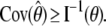
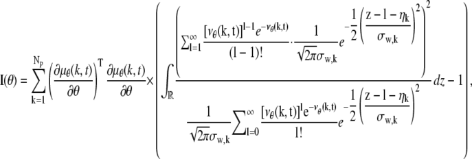
The depth discrimination capability of an optical microscope is characterized by how accurately the z position (i.e., depth) of a microscopic object can be determined from its image. To quantify this property, we adopt a stochastic framework and model the data acquired in an optical microscope as a spatio-temporal random process (44). The task of determining the 3D location of the object of interest is a parameter estimation problem, where an unbiased estimator is used to obtain an estimate of the 3D location. The performance of this estimator is given by the standard deviation of the location estimates assuming repeated experiments. According to the Cramer-Rao inequality (45,46), the (co)variance of any unbiased estimator  of an unknown parameter θ is always greater than or equal to the inverse Fisher information matrix, i.e.,
 |
(1) |
|---|
By definition, the Fisher information matrix provides a quantitative measure of the total information contained in the acquired data about the unknown parameter θ and is independent of how θ is estimated. Because the performance of an estimator is given in terms of its standard deviation, the above inequality implies that the square root (of the corresponding leading diagonal entry) of the inverse Fisher information matrix provides a lower bound to the performance of any unbiased estimator of θ. For the 3D location estimation problem carried out here, we define the 3D localization measure as the square root of the leading diagonal entry of the inverse Fisher information matrix corresponding to the z position.
Fisher information matrix for a conventional microscope
In this section, we provide expressions of the Fisher information matrix corresponding to the 3D location estimation problem for a conventional microscope. Here, the unknown parameter is set to θ = (_x_0, _y_0, _z_0) and the data consists of images acquired from a plane that is in focus with respect to the objective lens. First, we consider the best case imaging scenario, where the acquired data is not deteriorated by factors such as pixelation of the detector and extraneous noise sources. Here the data is assumed to consist of time points of the detected photons and the spatial coordinates at which the photons impact the detector. The analytical expression of the Fisher information matrix for the 3D location estimation problem is given by (44,47)
 |
(2) |
|---|
where θ = (_x_0, _y_0, _z_0) ∈ Θ denotes the 3D location, t denotes the exposure time, and Λ and  denote the photon detection rate and the image function of the object, respectively. An image function
  describes the image of an object at unit magnification that is located at (0, 0, _z_0) in the object space (44). The derivation of the above expression assumes that the photon detection rate Λ is independent of the 3D location, the image function
  is laterally symmetric for every
  i.e.,
i.e.,  and the partial derivative of
  with respect to _z_0 is laterally symmetric, i.e.,
  It should be pointed out that the above assumptions are typically satisfied for most 3D PSF models (48).
We next consider practical imaging conditions, where the acquired data consists of the number of photons detected at each pixel and is corrupted by extraneous noise sources. In many practical situations, in addition to estimating _x_0, _y_0, and _z_0, other parameters such as the photon detection rate and α are also estimated from the acquired data (for example, see section on MUMLA in Methods). Hence, in this context, we consider θ to be a general vector parameter. The data is modeled as a sequence of independent random variables  where _N_p denotes the total number of pixels in the image and
  k = 1,…,_N_p. The quantity Sθ,k (_B_k) is a Poisson random variable with mean μ θ(k, t) (β(k, t)) that models the detected photons from the object of interest (background) at the _k_th pixel; k = 1,…,_N_p, t denotes the exposure time; and _W_k is an independent Gaussian random variable with mean _η_k and standard deviation _σ_w,k that models the readout noise of the detector at the _k_th pixel, k = 1,…,_N_p. The analytical expression of the Fisher information matrix for a pixelated detector in the presence of extraneous noise sources is given by (34,44)
 |
(3) |
|---|
where θ ∈ Θ, ν θ(k, t) = μ θ(k, t) + β(k, t) for k = 1,…,_N_p, and θ ∈ Θ. Please see Appendix for details regarding the analytical expressions of μ θ and its partial derivatives.
Fisher information matrix for a MUM setup
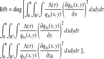
In a MUM setup, images of several distinct focal planes can be simultaneously acquired from the specimen. Each of the acquired images can be assumed to be statistically independent. If N distinct images are simultaneously acquired, the analytical expression of the Fisher information matrix corresponding to a general parameter estimation problem for a MUM setup is given by (also see (49))
 |
(4) |
|---|
where  k = 1,…,N, denotes the Fisher information matrix pertaining to the data acquired from the _k_th plane and the expression for
  is analogous to that given for a conventional microscope. In this work, the 3D location estimation for QDs is carried out by simultaneously imaging two distinct planes within the specimen. For this configuration, Eq. 4 becomes Itot(θ) =
 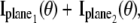 θ ∈ Θ. For the best case imaging scenario, the general expression for
  and
and  is analogous to that given in Eq. 2, except that Λ(τ), τ ≥ _t_0 will denote the photon detection rate per focal plane and in the expression for
  _z_0 will be replaced by _z_0 – _δz_f, where _δz_f denotes the focal plane spacing.
For practical imaging conditions (i.e., in the presence of pixelation and noise sources), the general expression for  and
and  is analogous to that of Eq. 3 and is given by
 |
(5) |
|---|
where  and j = 1, 2. Here, [_t_0,_t_] denotes the exposure time interval, _N_j denotes the number of pixels in the image acquired at the _j_th focal plane,
  and _β_j(k, t) denote the mean photon count from the object of interest and the background component, respectively, at the _k_th pixel in the image of the _j_th focal plane, and
  and
and  denote the mean and standard deviation of the readout noise, respectively, at the _k_th pixel in the image of the _j_th focal plane, for k = 1,…,_N_j and j = 1, 2. Please see Appendix for the analytical expressions of
  j = 1, 2 and its partial derivatives for the calculation of the Fisher information matrix for the two-plane MUM setup.
METHODS
MUM localization algorithm (MUMLA)
All data processing was carried out in MATLAB (The MathWorks, Natick, MA) and viewed using the Microscopy Image Analysis Tool (MIATool) software package (50). The 3D location of a QD was determined by fitting a pair of 3D PSFs to the data that was simultaneously acquired at the two distinct focal planes within the cell sample. From each focal plane image, a small region of interest (ROI) containing the QD image was selected. The pixel values in the acquired image correspond to digital units. Before curve fitting, the pixel values were converted to photon counts by subtracting the constant offset from each pixel value and then multiplying it by the conversion factor. The constant offset and the conversion factor were taken from the specification sheet provided by the camera manufacturer.
The intensity distributions of the ROIs in the two focal planes are modeled by image profiles  and
and  given by
  (k, t) =
  (k, t) + _B_1,k,
  (l, t) =
  (l, t) + _B_2,l, where
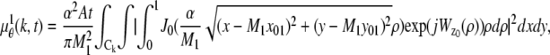 |
(6) |
|---|
 |
(7) |
|---|
_C_k (_C_l) denotes the region on the detector plane occupied by the _k_th (_l_th) pixel, and  l = 1,…, _N_2, and _N_1 and _N_2 denote the total number of pixels in the ROIs selected from plane 1 and plane 2, respectively.
In the above expressions _z_0 denotes the axial location of the point source; (_x_01, _y_01) and (_x_02, _y_02) denote the lateral (_X_-Y) location of the point source corresponding to focal plane 1 and focal plane 2, respectively; A denotes the photon detection rate for focal plane 1; t denotes the exposure time; c is a constant; _δz_f denotes the distance between the two focal planes in the object space; c is a constant; α = 2_πn_a/λ; _n_a denotes the numerical aperture of the objective lens; λ denotes the wavelength of the detected photons; _M_1 and _M_2 denote the lateral magnification corresponding to focal plane 1 and focal plane 2, respectively,  and
and  denote the background photon counts at each pixel in the ROIs of images from focal plane 1 and focal plane 2, respectively; and θ = (_x_01, _y_01, _x_02, _y_02, _z_0, α, A). The constant c specifies the fraction of the expected number of photons detected at focal plane 2, relative to focal plane 1. In our emission setup, the QD fluorescence signal that is collected by the objective lens is split into two paths by a 50:50 beam splitter. Further, the two focal plane images in the QD channel are imaged by two identical cameras operated at the same frame rate. Hence, we assume the expected number of photons detected from the QD to be the same in each focal plane image. Therefore, in all our calculations we set c = 1 (if a 30:70 beamsplitter is used and supposing focal plane 1 gets the 30% component, then c would be set to 2.33). The above expressions of
  and
and  make use of the Born and Wolf model of the 3D PSF (48) for which the phase aberration term
  is given by
 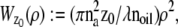 ρ ∈ [0, 1], where _n_oil denotes the refractive index of the immersion medium.
The focal plane spacing _δz_f was determined by conducting a bead imaging experiment as described in Prabhat et al. (41). In all of our MUM imaging experiments, one of the cameras was positioned at the design location, i.e., at the focal plane of the tube lens and the other camera was positioned at a nondesign location. Here, Eq. 6 (Eq. 7) is used to model the point-source image acquired by the camera at the design (nondesign) position. The magnification _M_1 is set to be equal to the magnification of the objective lens and _M_2 is determined in the following manner: An experiment was carried out where _z_-stack images of 100-nm tetraspeck fluorescent beads (Invitrogen, Carlsbad, CA) were acquired in a two-plane MUM setup. The in-focus image for each focal plane was chosen and the _X_-Y location of the beads was determined by fitting an Airy profile to the bead image. Then the distance between two arbitrarily chosen beads was calculated in each in-focus image and the ratio of the distances was then computed. The distance calculation was repeated for several bead pairs and the average of the ratio of the distances provided the ratio of the magnifications of the two focal planes. Using this, _M_1 and _M_2 were then determined.
For imaging data acquired from the stationary QD sample, the following protocol was used to estimate the z location: For each ROI, the background photon count was assumed to be constant for all pixels (i.e.,  and
and  ) and was estimated by taking the mean of the photon count from the four corner pixels of that ROI. The _X_-Y location coordinates (_x_01, _y_01) and (_x_02, _y_02) along with _z_0, α, and A were then determined by a global estimation procedure, which was implemented through the MATLAB optimization toolbox (lsqnonlin method). The estimation algorithm uses an iterative procedure to determine the unknown parameters by minimizing the error function, which returns the difference (i.e., error) between the model and the data at each iterate.
In the live-cell imaging data, the background significantly fluctuated across the ROI. Hence, the background photon counts  and
and  were estimated in the following manner: For each of the ROIs, a row (column) background template was constructed by fitting a straight line to the first and last pixel in each row (column) of that ROI. Then a mean background template was calculated by taking the (elementwise) average of the row and column background template, and this was used to determine the background pixel count for each pixel.
The _X_-Y location coordinates (_x_01, _y_01) and (_x_02, _y_02) were determined by independently fitting 2D Airy profiles to the ROIs by using estimation algorithms of the MATLAB optimization toolbox (lsqnonlin method). Here, the background photon count for each pixel was fixed and α and A were estimated along with the _X_-Y location coordinates. In some cases, curve fitting of the 2D Airy profile was feasible in only one of the ROIs. For example, such a scenario arises when the QD-Immunoglobulin G (IgG) molecule is on the membrane plane. Here, a strong signal can be seen in the image acquired from the membrane plane. However, the image from the top plane will appear to have little or no signal from the QD-IgG molecule, as it is out of focus with respect to that plane, resulting in an almost flat image profile. In such cases, one pair of the _X_-Y location coordinates is estimated through curve fitting. The estimated location coordinates are then mapped to the other focal plane to obtain an estimate of the other pair of _X_-Y location coordinates.
The z position of the point source was then estimated by simultaneously fitting both ROIs to 3D PSF profiles (Eqs. 6 and 7) using a global estimation procedure, which was implemented through the MATLAB optimization toolbox (lsqnonlin method). Here, the _X_-Y location coordinates (_x_01, _y_01) and (_x_02, _y_02), and the background photon counts were fixed, while α and A were estimated along with _z_0.
Both of the above described estimation procedures were tested on simulated data and the accuracy of the estimates was consistently close to the theoretically predicted accuracies for a range of z values. Here, we report the results of _z_-location determination from simulated data using the procedure described for the analysis of live-cell imaging data. As seen later in Figs. 5 c and 6 c, the 3D trajectories were generated by plotting the estimates of _x_01, _y_01, and _z_0. The trajectories do not include periods when the QD is blinking since the 3D location of the QD is not known. In Figs. 5 c and 6 c (later) and Supplementary Material Figs. S3 and S4 in Data S1, the _z_0 coordinates are shifted such that the smallest estimated value of _z_0 for that dataset is displayed as zero.
FIGURE 5.

Complex 3D trafficking itinerary of a QD-IgG molecule undergoing endocytosis. (a) Montages for FcRn and IgG channels along with the overlay displaying areas of interest of a transfected HMEC-1 cell with the time (in seconds) at which each image was acquired. Each row in the montage corresponds to a pair of images that was simultaneously acquired at the plasma membrane plane and at a plane that is 500 nm above the plasma membrane plane. In the overlay montage, FcRn is shown in green and IgG is shown in red. The QD-IgG molecule that is tracked is indicated by a white arrow. In some of the frames (e.g., see t = 28.05 s in the IgG channel), the image of the QD label visually appears as a very dim spot, but is detectable by MUMLA. The images in the IgG channels were acquired at a frame rate of 12 frames/s. The images shown are individual frames taken from Movie S1. Bar = 1 _μ_m. (b) Snapshot of the raw MUM data with the FcRn and IgG channels overlaid. The white box indicates the region in the cell that is shown in the montages. The red haze seen in the membrane and top planes is due to the presence of QD-IgG molecules in the imaging medium. Bar = 5 _μ_m. (c) 3D trajectory of the QD-IgG molecule. The trajectory is color-coded to indicate time. The color change from red to green to blue indicates increasing time. The QD-IgG positions indicated by arrows correspond to the images shown in panel a. The molecule is initially seen to be randomly diffusing on the plasma membrane. The endocytosis of the molecule is characterized by an abrupt change in its z location where the molecule moves inside the cell to a depth of 300 nm from the plasma membrane. After internalization, the molecule moves in a highly directed manner and takes an elaborate route to traffic deep inside the cell (800 nm from the plasma membrane) until it reaches a sorting endosome. The molecule briefly interacts with the sorting endosome, loops around it and then, after several repeated contacts, merges with the sorting endosome. See also Fig. S3 in Data S1 for a plot of the _z_0 coordinate as a function of time.
FIGURE 6.

Endocytosed QD-IgG molecule moves directly to the sorting endosome. (a) Montages for FcRn and IgG channels along with the overlay displaying areas of interest of a transfected HMEC-1 cell with the time (in seconds) at which each image was acquired. Each row in the montage corresponds to a pair of images that was simultaneously acquired at the plasma membrane plane and at a plane that is 500 nm above the plasma membrane plane. In the overlay montage, FcRn is shown in green and IgG is shown in red. The QD-IgG molecule that is tracked is indicated by a white arrow. The images in the QD channels were acquired at a frame rate of 12 frames/s. The images shown are individual frames taken from Movie S2. Bar = 1 _μ_m. (b) Snapshot of the raw MUM data with the FcRn and IgG channels overlaid. The white box indicates the region in the cell that is shown in the montages. The red haze seen in the membrane and top planes is due to the presence of QD-IgG molecules in the imaging medium. Bar = 5 _μ_m. (c) 3D trajectory of the QD-IgG molecule. The trajectory is color-coded to indicate time. The color change from red to green to blue indicates increasing time. The QD-IgG positions indicated by arrows correspond to the images shown in panel a. The QD-IgG molecule is initially observed to be diffusing on the plasma membrane for a significant period of time (t = 0–29.67 s). Before internalization, the molecule becomes stationary and then moves inside the cell in a highly directed manner toward a sorting endosome. See also Fig. S4 in Data S1 for a plot of the _z_0 coordinate as a function of time.
The diffusion coefficient of the QD-IgG molecule when on the plasma membrane was calculated from the mean-squared displacement (MSD) versus time lag curve. We consider a simple diffusion model in which the relation between the MSD and time-lag (t) is given by MSD(t) = 4_Dt_, where D denotes the diffusion coefficient (51). We use the standard approach in which a straight-line equation is fitted to the MSD versus time-lag plot and the diffusion coefficient is calculated from the slope of the fitted line (51).
Sample preparation
The human microvasculature endothelial cell line HMEC1.CDC (52), generously provided by F. Candal of the Centers for Disease Control (Atlanta, GA), was used for all experiments. Plasmids to express wild-type human FcRn tagged at the N-terminus with ecliptic pHluorin (pHluorin-FcRn), mutated human FcRn tagged at the C-terminus with mRFP or at the N-terminus with eGFP (FcRn_mut-mRFP or GFP-FcRn_mut), and human _β_2 microglobulin (h_β_2m) have been described previously (42,53), with the exception of GFP-FcRn_mut. GFP-FcRn_mut was engineered by inserting previously described mutations (54) into a wild-type human FcRn construct (GFP-FcRn) containing an in-frame N-terminal eGFP gene. GFP-FcRn was generated using an approach analogous to that described for the production of the pHluorin-FcRn expression plasmid (42). Quantum dot (QD) 655 coated with streptavidin and Alexa Fluor 555-labeled transferrin were purchased from Invitrogen. QD-IgG complexes were prepared as described previously (42).
HMEC1.CDC cells were transiently transfected with combinations of the above protein expression plasmids using Nucleofector technology (Amaxa Systems, Cologne, Germany) and were plated on either glass coverslips (Fisher Scientific, Pittsburgh, PA) or on MatTek dishes (MatTek, Ashland, MA). The cells were maintained in phenol red-free HAMS F12-K medium. For experimental verification of the MUM localization algorithm, two different stationary QD samples were prepared. Stationary QD sample 1 was prepared by pulsing FcRn-transfected HMEC cells with QD-IgG complexes (11 nM with respect to IgG) for 30 min at 37°C in a 5% CO2 incubator and then washed, fixed, and mounted on microscope slides. Stationary QD sample 2 was prepared by incubating 200 _μ_L of phosphate-buffered saline containing QDs (10 pM concentration) on a MatTek dish (MatTek). For live-cell imaging experiments, cells were incubated in medium (pH 7.2) containing QD-IgG complexes (11 nM with respect to IgG) and Alexa Fluor 555-labeled Transferrin (130 nM) in MatTek dishes and were subsequently imaged at 37°C.
MUM setup
MUM can be implemented in any standard optical microscope (41,42). Here, we provide the details of the implementation that was carried out on Zeiss microscopes (Carl Zeiss, Jena, Germany). Two different multifocal plane imaging configurations were used. The first configuration supports simultaneous imaging of two distinct planes within the specimen. A Zeiss dual video adaptor (Cat. No. 1058640000) was attached to the bottom port of a Zeiss Axiovert S100 microscope and two electron multiplying charge-coupled device (CCD) cameras (iXon DV887, Andor Technologies, South Windsor, CT) were used. Here, one of the cameras was attached to the video adaptor through a standard Zeiss camera-coupling adaptor (Cat. No. 4561059901). The other camera was attached to the video adaptor by using C-mount/spacer rings (Edmund Industrial Optics, Barrington, NJ) and a custom-machined camera-coupling adaptor that is similar to a standard Zeiss camera-coupling adaptor but of shorter length.
The second configuration supports simultaneous imaging of up to four distinct planes within the specimen. Here, a Zeiss video adaptor was first attached to the side port of a Zeiss Axiovert 200 microscope. Two Zeiss video adaptors were then concatenated by attaching each of them to the output ports of the first Zeiss video adaptor. Four high resolution CCD cameras (two ORCA-ER models and two C8484-05 models, Hamamatsu, Bridgewater, NJ) were attached to the output ports of the concatenated video adaptors by using C-mount/spacer rings and custom-machined camera coupling adaptors. To image more than four planes, the procedure described above can be repeated by concatenating additional video adaptors.
IMAGING EXPERIMENTS
Stationary QD sample imaging
Two types of stationary QD samples were imaged. Imaging of stationary QD sample 1 was carried out on a Zeiss Axiovert S100 microscope that supports simultaneous imaging of two distinct planes within the specimen (see Fig. S1 in Data S1 for additional details). The QD sample was illuminated in epifluorescence mode with a 488-nm laser line (Reliant 150M, Laser Physics, Salt Lake City, UT) and a 100×, 1.45 NA _α_-plan Fluar Zeiss objective lens was used. The fluorescence signal from the QDs were simultaneously acquired in two electron-multiplying CCD cameras (iXon DV887, Andor Technologies) which were synchronized through an external trigger pulse and were operated in conventional gain mode. The cameras were positioned such that the focal planes that they imaged inside the cell were 300-nm apart.
Images of stationary QD sample 2 were acquired using a Zeiss Axiovert 200 microscope that was modified to simultaneously image up to four distinct planes within the specimen (although only two planes were used in the current experiment). The QD sample was illuminated in epifluorescence mode with a 543-nm laser line (Research Electro Optics, Boulder, CO). A 63×, 1.2 NA C-Apochromat Zeiss objective was used. The fluorescence signal from the QDs were simultaneously acquired in two electron multiplying CCD cameras (iXon DV887, Andor Technologies), which were synchronized through an external trigger pulse and were operated in conventional gain mode. The cameras were positioned such that the focal planes that they imaged were 1200-nm apart.
Live-cell imaging
Images of live cells were acquired using a Zeiss Axiovert 200 microscope that was modified to simultaneously image up to four distinct planes within the specimen. The cell sample was concurrently illuminated in epifluorescence mode with a 543-nm laser line (Research Electro Optics) and in TIRF mode with a 488-nm laser line (Reliant 150M, Laser Physics). A 100×, 1.45 NA _α_-plan Fluar Zeiss objective lens was used. Both laser lines continuously illuminated the sample throughout the duration of the experiment. Four high-resolution CCD cameras (two C8484-05 models and two ORCA-ER models, Hamamatsu) were used to capture the data. The cell was simultaneously imaged in two planes, i.e., the membrane plane and a plane that is 500 nm above the membrane plane and inside the cell. In the membrane plane, the fluorescence signal from pHluorin-labeled FcRn and QD-labeled IgG were captured in two separate cameras. In the top plane, the signal from mRFP-labeled FcRn and Alexa 555-labeled transferrin were captured in the third camera and the signal from QD-labeled IgG was captured in the fourth camera. (Please see Fig. S2 in Data S1 for additional details regarding the camera exposure times and the various filters used in the emission light path.)
RESULTS
Estimating 3D position using MUMLA
MUM was developed for 3D tracking of subcellular objects in live cells (41,42). To use MUM for 3D single molecule/particle tracking applications, it is necessary to be able to determine the 3D position of the particle at each point in time. For this, we have developed the MUM localization algorithm (MUMLA). For a two-plane MUM setup, MUMLA is based on the following approach: for each pair of point source images I1 and I2 acquired in the two MUM planes, the 3D point-spread functions PSF1 and PSF2 (Eqs. 6 and 7) are simultaneously fitted to obtain the point source position that best matches the acquired data (see Methods for details). The fact that the algorithm can rely on information not only from one defocus level but also from two provides significant additional constraints to the estimation problem that result in an improved performance.
We tested MUMLA through Monte Carlo simulations as well as experimental data. For simulations, images of a point source were generated for a two-plane MUM setup for different values of _z_0 assuming practical imaging conditions (see Table 1 for details). Fig. 2 a shows the results of the MUMLA estimates for the simulated data. From the figure, we see that the algorithm correctly estimates the z position of the point source for a range of _z_0 values (0–500 nm). Table 1 lists the true value of _z_0 along with the mean and standard deviation of the _z_0 estimates from simulated data. Note that even for very small _z_0 values (e.g., _z_0 = 0 nm), the z position can be determined. In the simulated data, the average photon count of the point source in each focal plane was set to 1000 photons. For this imaging condition, MUMLA recovered the z position of the point source with an accuracy (standard deviation) of 20–30 nm for _z_0 values in the range of 0–500 nm.
TABLE 1.
Verification of the improved depth discrimination capability of MUM
| True value of _z_0 [nm] | Mean value of _z_0 estimates [nm] | SD of _z_0 estimates [nm] | 3D localization measure of _z_0 [nm] |
|---|---|---|---|
| 0 | −3.74 | 24.67 | 26.23 |
| 50 | 45.40 | 25.49 | 24.58 |
| 100 | 98.70 | 22.43 | 23.19 |
| 150 | 152.52 | 25.22 | 22.14 |
| 200 | 195.45 | 20.87 | 21.48 |
| 250 | 247.39 | 22.98 | 21.24 |
| 300 | 299.72 | 22.27 | 21.45 |
| 350 | 351.81 | 23.82 | 22.10 |
| 400 | 405.33 | 24.41 | 23.16 |
| 450 | 457.11 | 28.49 | 24.58 |
| 500 | 506.80 | 29.79 | 26.30 |
FIGURE 2.

Verification of MUMLA. (a) Results of _z_-position estimates from simulated data for a QD label. Two-plane MUM images were simulated for different _z_-position values, where the plane spacing between the two focal planes in the object space was assumed to be 500 nm. The z position from the simulated data was obtained using MUMLA. The plot shows the estimates of z position (°) at each value of _z_0 along with the true value of _z_0 (—). (b and c) Results of _z_-position estimates of two QD labels from experimental data. For panel b, a cell sample (stationary QD sample 1) that was pulsed with QD labeled IgG molecules and fixed was imaged in a two-plane MUM setup (focal plane spacing in object space = 300 nm). The objective was moved in 50-nm steps with a piezo-nanopositioner and at each piezo position several images of the specimen was acquired. The z position of an arbitrarily chosen QD was determined using MUMLA. The plot shows the estimates of z position (°) for one of the QDs at various piezo positions along with the mean value of the _z_-position estimates for each piezo position (—). For panel c, sparsely dispersed QDs on a cover glass (stationary QD sample 2) were imaged in a two-plane MUM setup (focal plane spacing in object space = 1.2 _μ_m). The objective was moved in 200-nm steps with a piezo-nanopositioner and at each piezo position several images of the specimen were acquired. The z position of an arbitrarily chosen QD was determined using MUMLA in combination with the calibration plot (see Results for details). The plot shows the estimates of z position (°) for one of the QDs at various piezo positions along with the mean value of the _z_-position estimates for each piezo position (—).
The experimental data was acquired by imaging stationary QD samples. To obtain images of QDs with different _z_0 values, the objective lens was moved with a piezo-nanopositioner (PI-USA, Auburn, MA) in either 50-nm steps (stationary QD sample 1) or 200-nm steps (stationary QD sample 2) and at each piezo position several images of the two focal planes were simultaneously captured. The z position of the QD was then determined by using MUMLA. Because of stage drift problems, two different step sizes were used to obtain images of the QD over different spatial ranges. In particular, the 50-nm step size was used to obtain images over a spatial range of 300 nm and the 200-nm step size was used to obtain images over a spatial range of 2.4 _μ_m.
Fig. 2 b shows the plot of the z location estimates for a QD over a small range of _z_0 values (_z_0 = −27 nm to 290 nm) illustrating the 50-nm stepwise movement of the piezo-nanopositioner. Here, the difference between the successive defocus steps are 43.1 nm, 55.8 nm, 55.2 nm, 60.6 nm, 53 nm, and 50.3 nm, which is in reasonable agreement with the 50 nm step size of the piezo-nanopositioner (see Table 2). Table 2 lists the mean and standard deviation of the z position estimates for one of the QDs. Table 2 also lists the step level, which is the difference between the average z position estimates between the two successive piezo positions. Here, an average of 4000 photons were acquired from the QD at each focal plane and we see that the z position of the QD was determined with an accuracy of 13–15 nm.
TABLE 2.
Experimental verification of MUMLA
| Focus level | Mean value of _z_0 estimates [nm] | SD of _z_0 estimates [nm] | 3D localization measure of _z_0 [nm] | Step size leveln–leveln−1 [nm] |
|---|---|---|---|---|
| 1 | −27.2 | 12.70 | 13.42 | — |
| 2 | 15.9 | 16.90 | 14.11 | 43.1 |
| 3 | 71.7 | 17.68 | 14.40 | 55.8 |
| 4 | 126.9 | 11.10 | 14.42 | 55.2 |
| 5 | 187.5 | 16.04 | 15.16 | 60.6 |
| 6 | 240.5 | 20.40 | 15.04 | 53.0 |
| 7 | 290.8 | 16.64 | 14.91 | 50.3 |
Fig. 2, a and b, shows that MUMLA can recover the _z_-position values in the range of 0–500 nm. To verify the validity of MUMLA at depths beyond 500 nm, stationary QD sample 2 was imaged (see Methods). A QD was arbitrarily chosen from the acquired data and its z position at each focus level was estimated using MUMLA. A calibration plot was generated that relates the focus level of the objective lens to the QD z position. Then images of another QD molecule were analyzed through MUMLA and using the calibration graph as reference, the focus levels were recovered. Fig. 2 c shows the results of the recovered _z_0 coordinate estimates for one such QD illustrating the 200-nm stepwise movement of the piezo-nanopositioner (see Table 3). From the figure we see that MUMLA correctly recovers the piezo step sizes over a spatial range of 2.4 _μ_m. Note that this approach not only works at large depths but also at depths when the QD is close to _z_0 = 0. In this experiment, z position estimation beyond 2.4 _μ_m was not feasible, since in one direction the limitation was due to insufficient number of photons above the background in the acquired data while in the other direction the limitation was due to the lack of symmetry of the 3D PSF profile about the focal plane. Table 3 lists the mean and standard deviation of the z position estimates for one such QD. This table also lists the recovered piezo step size, which is in reasonable agreement to the 200-nm step size. Note here that the accuracy of the z position estimates varies from 12 to 60 nm. This large variation in the accuracy can be attributed in part to the wide spatial range over which the z positions were being determined.
TABLE 3.
Experimental verification of MUMLA for a large spatial range
| Focus level | Mean value of _z_0 estimates [nm] | SD of _z_0 estimates [nm] | 3D localization measure of _z_0 [nm] | Step size leveln–leveln−1 [nm] |
|---|---|---|---|---|
| 1 | −1154.6 | 12.31 | 17.42 | — |
| 2 | −957.7 | 43.56 | 19.57 | 201.9 |
| 3 | −716.4 | 42.87 | 21.88 | 236.3 |
| 4 | −548.6 | 60.89 | 27.30 | 257.8 |
| 5 | −245.3 | 23.38 | 22.93 | 213.4 |
| 6 | −60.5 | 28.68 | 21.75 | 184.7 |
| 7 | 155.7 | 27.96 | 20.74 | 216.6 |
| 8 | 390.6 | 26.91 | 19.24 | 234.9 |
| 9 | 638.3 | 29.80 | 19.23 | 247.7 |
| 10 | 881.7 | 29.95 | 20.52 | 243.4 |
| 11 | 1039.3 | 40.13 | 25.70 | 187.6 |
| 12 | 1254.1 | 56.14 | 29.86 | 184.7 |
It should be pointed out that in Tables 2 and 3, the discrepancy between the calculated step size and the actual step size can in part be attributed to the positioning accuracy of the piezo, which, according to the manufacturer, is in the range of ±10–20 nm.
MUMLA and _z_-localization accuracy
In the previous section, we showed that MUMLA correctly recovers the piezo position from the QD images for a wide spatial range. A common question that arises when designing estimation algorithms is what is the best possible accuracy with which the unknown parameter of interest can be determined and more importantly, whether a given algorithm can attain this accuracy. To address this issue in the context of MUMLA, we have carried out a rigorous statistical analysis, the details of which are given in the Theory section (see above). Our approach is to quantify the total information contained in the acquired data about the z position of the point source. This quantification is done by calculating the Fisher information matrix for the underlying estimation problem of determining the z position of the point source. We then make use of a well-known result in statistical estimation theory called the Cramer-Rao inequality (45) which, when applied to our problem, implies that the accuracy (i.e., standard deviation) of the _z_-position estimates obtained using any reasonable estimation algorithm is bounded from below by the square root of the inverse Fisher information matrix. Stated otherwise, the square root of the inverse Fisher information matrix provides the best possible accuracy with which the z position of the point source can be determined for a given dataset. It should be pointed out that the Fisher information matrix is independent of how the unknown parameter (i.e., the z position) is estimated and only depends on the statistical description of the acquired data. Hence, we define the square root of the inverse Fisher information matrix corresponding to the _z_-position estimation problem as the 3D localization measure of _z_0.
To verify whether MUMLA indeed attains the best possible accuracy, we have calculated the 3D localization measure of _z_0 for the simulated and the experimental datasets and the results of our calculations are listed in Tables 1–3. From the tables we see that for each dataset the accuracy (standard deviation) of the _z_-position estimates obtained using MUMLA comes consistently close to the 3D localization measure of _z_0 for a wide range of _z_0 values. This shows that MUMLA provides the best possible accuracy for determining the z position of the QD. Note that in some of the datasets the accuracy of the _z_-position estimates is bigger than the 3D localization measure, while in other datasets the accuracy of the _z_-position estimates is smaller than the 3D localization measure. This variability is due to the fact that the accuracy was calculated from a small number (12–15) of _z_-position estimates, as only a limited number of MUM images were acquired at each piezo position to minimize the influence of stage drift on the acquired data. However, if a larger number of images were collected then we expect the accuracy of the _z_-position estimates to more closely follow the 3D localization measure.
The 3D localization measure results given in Tables 1–3 are based on _z_-position estimates that are obtained from a single MUM image, i.e., a pair of images that are simultaneously acquired at the two focal planes. If we take into account the full data set for a given piezo position, i.e., all the MUM images acquired at that piezo position, then the 3D localization measure calculations predict that the QD can be localized with significantly higher accuracy. For example, in Table 2, consider focus level 3 where the mean of the _z_-position estimates is _z_0 = 71.7 nm. For this _z_0 value, the 3D localization measure predicts an accuracy of 14.4 nm when only one MUM image is used to determine the z position. On the other hand, if all the MUM images are used that are acquired at that focus level, then the 3D localization measure predicts an accuracy of 3.9 nm in determining the z position.
Depth discrimination capability of MUM
The depth discrimination property of an optical microscope is an important factor in determining its capability for 3D imaging and tracking applications. In a conventional microscope, even for a high numerical aperture objective, the image of a point source does not change appreciably if the point source is moved several hundred nanometers from its focus position (Fig. 1 b, bottom row). This makes it extraordinarily difficult to determine the axial, i.e., z position, of the point source with a conventional microscope. To quantify the influence of depth discrimination on the _z_-localization accuracy of a point source, we calculate the 3D localization measure of _z_0 for a conventional microscope for practical imaging conditions (see Theory for details). The 3D localization measure provides a quantitative measure of how accurately the location of the point source can be determined. A small numerical value of the 3D localization measure implies very high accuracy in determining the location, while a large numerical value of the 3D localization measure implies very poor accuracy in determining the location. Fig. 1 c shows the 3D localization measure of _z_0 for a point source that is imaged in a conventional microscope. From the figure, we see that when the point source is close to the plane of focus, e.g., _z_0 ≤ 250 nm, the 3D localization measure predicts very poor accuracy in estimating the z position. For example, for _z_0 = 250 nm, the 3D localization measure predicts an accuracy of 31.79 nm and for _z_0 = 5 nm, the 3D localization measure predicts an accuracy of >150 nm, when 2000 photons are collected from the point source. Thus, in a conventional microscope, it is problematic to carry out 3D tracking when the point source is close to the plane of focus.
In MUM, images of the point source are simultaneously acquired at different focus levels. These images give additional information that can be used to constrain the z position of the point source (see Fig. 1 b). This constraining information largely overcomes the depth discrimination problem near the focus. As shown in Fig. 1 c, we see that for a two-plane MUM setup (focal plane spacing = 500 nm), the 3D localization measure predicts consistently better accuracy in determining the z position of the point source when compared to a conventional microscope. For example, for _z_0 values in the range of 0–250 nm, the 3D localization measure of _z_0 predicts an accuracy of 20–25 nm in determining the z position when 1000 photons are collected from the point source at each focal plane.
Note that for the MUM setup, the predicted _z_-position accuracy is relatively constant for a range of _z_0 values (e.g., _z_0 = 0–1000 nm), which is in contrast to a conventional microscope where the predicted _z_-position accuracy varies over a wide range of values. This implies that the z location of a point source can be determined with relatively the same level of accuracy for a range of _z_0 values, which is favorable for 3D tracking applications. In particular, the finite value of the 3D localization measure for _z_0 values close to zero implies that the z position of the point source can be accurately determined in a MUM setup when the point source is near the plane of focus.
Consistent with earlier results in localization studies (34,35,44,47), our analysis shows that the accuracy with which the z position of a point source can be determined depends on the number of photons that are collected per exposure (see Fig. 1 c and Fig. 3). In the above example, for the two-plane MUM setup, if we detected 2000 photons from the point source in each plane, then our result predicts an accuracy of 14–18 nm for _z_0 values in the range of 0–600 nm.
FIGURE 3.

Effect of signal and noise statistics on the 3D localization measure. The figure shows the variation of the 3D localization measure of _z_0 for a two-plane MUM setup as a function of the expected number of detected photons per plane for readout noise levels of 6 _e_−/pixel (°) and 15 _e_−/pixel (⋄). In all the plots, the photon detection rate is set to 5000 photons/s per plane, the background rate is set to 200 photons/pixel/s per plane, and the _x_-axis range corresponds to an exposure time range of t = 0.1–2 s. All other numerical values are identical to those used in Fig. 1 c.
Our 3D localization measure calculations explicitly take into account the shot noise characteristics of the signal from the point source. Specifically, the detected photon counts from the point source in the acquired data are modeled as independent Poisson random variables. Additionally, we take into account the presence of additive noise sources and the effects of pixelation in the data. We consider two additive noise sources, i.e., additive Poisson and additive Gaussian noise sources. The Poisson noise component is used to model the effects of background photons that arise, for example, due to autofluorescence of the cell-sample/imaging-buffer and scattered photons. The Gaussian noise component is used to model the measurement noise that arises, for example, during the readout process in the imaging detector.
Fig. 3 shows the behavior of the 3D localization measure of _z_0 for various signal and noise levels. In particular, we have considered two different readout noise levels (6 _e_− per pixel and 15 _e_− per pixel root-mean squared) and several different signal and background levels. From the figure, we see that the 3D localization measure of _z_0 predicts consistently worse accuracy for the higher readout noise level. Note that the difference in the predicted accuracy between the two readout noise levels begins to decrease as the number of signal photons increases.
Previously our group (34) and others (35,55) have shown the dependence of the detector pixel size on the accuracy with which the 2D location of a point object can be determined. Here we have extended this analysis to the 3D localization problem. Specifically, we calculated the 3D localization measure of _z_0 for a MUM setup for different pixel sizes and this is shown in Fig. 4. Here, we set the background component to be zero, and the number of detected photons and the readout noise to be the same for all pixel sizes. From the figure, we see that as the pixel size increases the 3D localization measure of _z_0 first decreases, but then increases. At small pixel sizes, the image profile of the point source will be spatially well sampled. However, due to the small size of the pixel, only a few photons will be collected at each pixel from the point source. As a result, the readout noise component becomes significant in each pixel, thereby resulting in poorer accuracy. As the pixel size increases, more photons will be collected in each pixel from the point source and thus the accuracy becomes better. For very large pixel sizes, a sufficient number of photons will be collected in each pixel but the profile will be poorly sampled spatially. This results in inadequate spatial information and thus the accuracy becomes worse. An analogous behavior was also observed for the 2D localization problem as reported in the literature (34,35,55).
FIGURE 4.

Effect of detector pixel size on the 3D localization measure. The figure shows the variation of the 3D localization measure of _z_0 as a function of the detector pixel size for a two-plane MUM setup for _z_-position values of 250 nm (⋄) and 150 nm (*). We assume the pixel size and the readout noise statistics to be the same for both focal plane images. In all the plots, the background component is set to zero; the standard deviation of the readout noise is set to 6 _e_−/pixel; the exposure time is set to 0.2 s; the photon detection rate is set to 5000 photons/s per plane; and the pixel array is set to 500 × 500 _μ_m. The pixel sizes were chosen such that the pixel array consists of an odd number of rows and columns. All other numerical values are identical to those used in Fig. 1 c.
3D QD tracking in live cells
Immunoglobulin G (IgG) molecules represent an essential component of the humoral immune system. IgG molecules mediate the neutralization and/or clearance of pathogenic components in the body. The recent past has witnessed the rapidly expanding use of IgG molecules as therapeutic and diagnostic agents (56). The study of the intracellular trafficking pathways of IgGs is therefore not only of importance for the understanding of fundamental aspects of the immune system, but also to investigate the mechanisms of IgG-based therapeutics/diagnostics. Using MUM, we have imaged for the first time the 3D trafficking pathway of single QD-labeled IgG molecules from the plasma membrane to the interaction with sorting endosomes at a depth of 1 _μ_m within the cell, which is not possible with current imaging technologies. In particular, the 1-_μ_m imaging depth is well beyond the reach of the TIRF microscopy that is typically used for detailed studies of endocytic events near the plasma membrane. Human endothelial cells were transiently transfected with fusion protein constructs encoding FcRn (FcRn-pHluorin and FcRn-mRFP, see Methods for details). FcRn is a specific receptor for IgG that is expressed in many cell types (43). FcRn is predominantly localized in endosomal compartments inside the cell and is also present on the cell surface (5,53). Here, we use fluorescently tagged FcRn to label the cellular structures as well as to facilitate receptor-mediated endocytosis of QD-IgGs in cells. The dynamics of FcRn and IgG were simultaneously imaged at the membrane plane (via TIRF illumination) as well as at a focal plane in the cell interior (via epifluorescence illumination) at which the sorting endosomes were in focus (500 nm from the cell membrane).
Fig. 5 a shows a montage of FcRn and IgG channels that were simultaneously acquired at two focal planes in the cell. In the top plane images of the FcRn channel, a ring-shaped structure can be observed, which is a sorting endosome (see (53) for details regarding the identification of a sorting endosome). In this dataset, the ring-shaped structure is also observed in the IgG channel due to the presence of QD-IgGs in the sorting endosome. Fig. 5 c shows a track of a QD-IgG molecule that was obtained by analyzing the MUM data using MUMLA. This track exhibits highly complex dynamics on the endocytic pathway. The QD-IgG molecule is initially observed on the plasma membrane and is randomly diffusing (D = 0.001–0.005 _μ_m2/s, in agreement with previous studies on membrane receptor dynamics (24,57–59)). During this phase, the QD can be seen only in the membrane plane image (Fig. 5 a, t = 1.79 s) and the mean value of its z location is 160 nm. Before internalization, the molecule becomes stationary for 0.7 s. The endocytosis phase is characterized by an abrupt change in the z location of the molecule, where it moves inside the cell by 360 nm from the plasma membrane (also see Fig. S3 in the Data S1). During this phase, the QD can be seen in both the top plane and the membrane plane (Fig. 5 a, t = 28.05 s). The molecule briefly stays at the same depth, then comes very close to the plasma membrane and starts to move in a highly directed manner (Fig. 5 a, t = 31.03 s). It then moves a distance of 17.1 _μ_m laterally across and inside the cell to reach a depth of 800 nm from the plasma membrane to come in close proximity to a sorting endosome. During this phase, the molecule moves with an average 3D speed of 2.5 _μ_m/s, suggesting that the movement is directed on microtubules and molecular motors (60). It then briefly interacts with the sorting endosome during which the QD is seen only in the top plane (Fig. 5 a, t = 36.47 s). The QD-IgG molecule then loops around the sorting endosome with an average 3D speed of 2.1 _μ_m/s and covers a distance of 8.7 _μ_m. Here, the molecule moves toward the plasma membrane to a depth of 365 nm and then moves back inside the cell to a depth of 695 nm from the plasma membrane to interact with the sorting endosome again. The molecule makes several repeated contacts with the sorting endosome before merging with its membrane. During this phase, the QD is again seen only in the top plane (Fig. 5 a, t = 56.19 s).
Not all pathways are as complex as that seen in Fig. 5. Fig. 6 shows the 3D trajectory of a QD-IgG molecule, which, after internalization, moves directly to a sorting endosome. Analogous to the dynamics seen in Fig. 5, the QD-IgG molecule is initially observed on the plasma membrane where it exhibits diffusive behavior (D = 0.002–0.006 _μ_m2/s). During this phase, the QD is seen only on the membrane plane (Fig. 6 a, t = 0.68 s) and the mean value of its z location is 169 nm. It diffuses on the plasma membrane plane for a significant period of time (t = 0–29.67 s). Before internalization, the molecule becomes stationary for 0.5 s and then moves inside the cell in a highly directed manner toward a sorting endosome. During this phase, the QD travels a distance of 2.72 _μ_m and reaches a depth of 610 nm from the plasma membrane. When the QD is close to the sorting endosome, it can be seen only in the top plane (Fig. 6 a, t = 31.79 s) (also see Fig. S4 in Data S1). It should be pointed out that in both figures, we observed blinking of the QD throughout its trajectory, confirming that individual QDs were tracked. The blinking behavior did not interfere with the tracking of QDs, since when blinking occurred the QDs were sufficiently isolated and hence they were unambiguously identified when they appeared again in the image. In the live-cell data shown here, we collected an average of 1000 photons per plane from the QD and we were able to localize the QD-IgG molecule with an accuracy ranging from 20 to 30 nm (6–12 nm) along the _z_-(_x_-,_y_-)direction.
DISCUSSION
The study of 3D intracellular trafficking pathways is important for understanding protein dynamics in cells. Conventional microscopy-based imaging techniques are not well suited for studying 3D intracellular dynamics, since only one focal plane can be imaged at any given point in time. As a result, when the cell-sample is being imaged in one focal plane, important events occurring in other planes can be missed. To overcome these shortcomings, we had developed MUM to simultaneously image multiple focal planes in a sample (41). This enables us to track subcellular objects in three dimensions in a live cell environment. Using MUM, we had studied the transport itineraries of IgG molecules in the exocytic pathway in live cells (42). These results provided qualitative data, i.e., simultaneous images of IgG transport at different focal planes in a cell. In the current work, we present a methodology for the quantitative 3D tracking of nanoparticle/QD-tagged proteins in live cells. Specifically, we have developed a 3D localization algorithm MUMLA to determine the position of a point object in three dimensions from MUM images.
We tested MUMLA on simulated as well as experimental data. Of importance is the verification that the estimates obtained with MUMLA are indeed the correct ones (i.e., unbiased). We have shown that MUMLA correctly recovers the _z_-position estimates (simulated data) and correctly infers the step sizes (experimental data) for a wide spatial range (∼2.5 _μ_m). A fundamental question that arises when developing estimation algorithms is what is the best possible accuracy with which the unknown parameters of interest can be determined, and importantly whether the proposed algorithm attains this accuracy. Here, to address these issues, we have carried out a statistical analysis based on the Fisher information matrix, which provides a quantitative measure of the total information contained in the acquired data about the parameters that we wish to estimate. We have derived mathematical expressions to calculate the Fisher information matrix for the three position parameters of a point object for a MUM imaging configuration (and also for a conventional microscope configuration). Further, using these formulae we calculate the 3D localization measure of _z_0, which provides a limit to the localization accuracy of the z coordinate.
We have shown that the standard deviation (accuracy) of the z estimates obtained using MUMLA comes consistently close to the 3D localization measure of _z_0 for a wide range of z values. It is important to note that the Fisher information matrix-based formula is independent of how the location coordinates are estimated and only depends on the statistical description of the acquired data. Thus, the 3D localization measure provides a benchmark against which different algorithms can be compared. Typically, in parameter estimation problems, only one or a few algorithms attains this benchmark. In this case, the close agreement between the accuracy of MUMLA and the 3D localization measure shows that indeed MUMLA is the best algorithm for determining the z position of the point object for a given dataset.
MUMLA does not have any intrinsic limitations on the spatial range over which it is applicable. For the specific experimental configuration used here, MUMLA was able to recover the z position up to a depth of 2.5 _μ_m. Should the dynamics of interest span a greater depth, the methodology presented here can be extended in a straightforward fashion, for example, by simultaneously imaging more than two focal planes and then deducing the z position from the resulting dataset. In contrast, other 3D localization approaches such as the use of cylindrical lenses (19,20) and the use of out-of-focus rings (16,17) (see below for additional details) have intrinsic limitations on the spatial range over which they are applicable. For instance, in Holtzer et al. (20) it was reported that the cylindrical-lens-based approach is limited to tracking point objects up to a depth of ≤1 _μ_m.
To demonstrate the applicability of MUMLA to real-world biological problems, we tracked single QD-IgG molecules in three dimensions along the endocytic pathway in live cells. We imaged the trafficking itinerary of single QD-IgG molecules starting from the plasma membrane and going all the way to a sorting endosome deep inside the cell. It should be pointed out that the intracellular trafficking pathways are poorly understood and this can be partly attributed to the lack of an appropriate methodology to track subcellular objects and single molecules in three dimensions inside a cell. The results of our live-cell imaging data demonstrate that MUMLA can be applied to address such important cell biological problems.
An important requirement for 3D single particle tracking is that the particle should be continuously imaged when it undergoes complex 3D dynamics. Conventional microscopy-based imaging approaches can only image one focal plane at any given point in time. In this case, 3D localization of single particles can be carried out using _z_-stack images, which are obtained by sequentially moving the objective lens in discrete steps with a focusing device and acquiring the image of the different focal planes. However, due to the relatively slow speed of focusing devices when compared to many of the intracellular dynamics, 3D localization approaches that infer the z position from _z_-stack images (11,13,22) are limited in terms of the acquisition speed and in the type of events that they can track. The MUM imaging approach, on the other hand, simultaneously images multiple focal planes within the sample. This eliminates the need to move the objective to observe the dynamic events occurring inside the cell in three dimensions. In this way, MUM enables the imaging of complex 3D intracellular dynamics at high temporal precision. This in conjunction with MUMLA provides the full 3D trajectories of events occurring inside a cell.
Another important aspect of 3D single particle tracking is whether the 3D location of a particle can be determined when it is at a certain depth and how accurately this can be done. One of the major limitations of conventional microscopes in the context of 3D localization is their poor depth discrimination capability. That is, it is extraordinarily difficult to determine the z position of the point object when it is close to the plane of focus. Here, we have shown that the 3D localization measure of _z_0 for a conventional microscope configuration becomes worse when the point object is close to the plane of focus thereby predicting poor accuracy in determining the z position. Thus, 3D tracking of single particles near the focus can be problematic with conventional microscopy-based imaging techniques (18). On the other hand, for a MUM imaging configuration, the 3D localization measure of _z_0 predicts consistently better accuracy in determining the z position of the point source when it is close to the plane of focus. Thus, by using the MUM imaging configuration, the depth discrimination problem can be overcome. In this work, this has enabled us to track QDs with relatively high accuracy when they are close to the plane of focus.
Consistent with previous reports on the 2D localization problem (34,35,55), our statistical analysis shows the 3D localization measure of _z_0 depends on the number of detected photons. We have shown that as the number of detected photons increases, the predicted accuracy in the z position improves. We have also analyzed the effect of pixel size on the 3D localization measure of _z_0 for a MUM imaging configuration under typical experimental conditions. These results can be employed in several ways in the context of 3D single particle tracking. For example, for a concrete experimental configuration we can evaluate the 3D localization measure of _z_0 for various _z_-position values. In this way, we can determine the feasibility of carrying out a particular experiment for a given imaging configuration. Further, by calculating the 3D localization measure for different combinations of signal, background, readout noise levels and pixel sizes we can determine a priori the most optimal imaging configuration for achieving high _z_-localization accuracy.
To use MUMLA on experimental data, it is necessary to know the distance between the two focal planes in the object space, which needs to be experimentally determined. An error in the determination of the focal plane distance could result in biased _z_-position estimates. In the extreme case, an incorrect focal plane spacing would result in poor fits of the model profiles to the experimental data. Similarly, MUMLA also requires the lateral magnifications of the two focal planes to be known, which may need to be experimentally determined. An error in the calculation of the magnification values could also lead to biased z estimates. In all of our experiments, one of the focal planes coincided with the focal plane of the objective lens. Hence, the lateral magnification for this plane was set to the magnification of the objective lens and this left us with the determination of only one magnification value.
It should be pointed out that MUMLA is independent of the specific experimental configuration that is used to simultaneously acquire the different focal plane images. In our experimental setup, we imaged the QD-IgG dynamics by capturing the QD signal at two focal planes in the cell sample on two cameras and at the same time, we also imaged the receptor (FcRn) dynamics by capturing the FcRn signal at the same focal planes on two other cameras. However, other MUM imaging configurations are also possible. For instance, instead of projecting the two focal plane images on two cameras, it can also be projected onto the chip of a single camera, as reported in Toprak et al. (17).
An important characteristic of MUMLA is the way in which it uses the MUM imaging data to determine the z position. Given two focal plane images of a point object, a question arises as to what is the best way in which the data can be used to extract the 3D position. Our statistical analysis shows that the use of both focal plane images provides consistently better accuracy in determining the z position when compared to using only one focal plane image, especially when the point object is near the focus. MUMLA infers the z position of a point object from two focal plane images. In particular, the use of two focal plane images instead one provides additional data concerning the z location of the point source. In our implementation of MUMLA, we carry out a global estimation using both focal images, where the additional data provides constraining information regarding the z position. This results in the observed superior performance of MUMLA, especially for _z_-position estimation when the point object is close to the focus. The localization algorithm used in Toprak et al. (17) was originally proposed by Speidel et al. (16), and makes use of only one focal plane image, in particular the out-of-focus image of the point object, to deduce the z position. Therefore, this algorithm does not make use of the constraining information that is available in the second focal plane image.
The localization algorithm of Speidel et al. imposes a stringent requirement of the presence of out-of-focus rings in the acquired image, which is satisfied only when the point object is at certain depths. As a result, the algorithm is limited to tracking point objects only at these depths. Even within this specific depth range, the algorithm poses several limitations. For instance, a large number of photons need to be collected to detect the out-of-focus rings in the image and this is often not possible due to several practical limitations. Moreover, it was reported in Toprak et al. (17) that this algorithm cannot track QD. On the other hand, MUMLA does not impose any constraints such as the presence of out-of-focus rings, which makes it applicable to a wide range of depths. In particular, our algorithm is not only effective in accurately determining the z position when the point source is close to or at the plane of focus but also for large defocus values. Further, as shown here, MUMLA can be used to track QDs at very high spatial and temporal precision.
In this study, the use of QD label was motivated by its generally favorable photophysical properties such as brightness and photostability. In particular, these properties enabled us to track important biological events in three dimensions for extended periods of time, allowing us to collect a sufficient number of photons per frame and image at relatively fast frame rates (12 frames/s). We believe that this would have otherwise not been possible with organic dyes and fluorescent proteins. A common concern that arises with QD labels is their size, which is relatively large when compared to conventional fluorophores. This could affect binding properties or the biological activity of the molecule that is tagged with the QD (“tail wagging the dog” problem (61)). Further, because of the QD size, it is important to keep in mind that it is the position of the label that is being determined rather than the position of the molecule that is tagged. Unfortunately, these issues typically show up not only when using QD labels, but also in other single particle experiments that use gold or fluorescent beads.
MUMLA is not limited to QD tracking. For example, the 3D tracking of vesicles and viruses poses very similar problems that can be addressed with the same approach that we have described. For the tracking of larger objects, the fitting of PSF models is not appropriate but can be replaced by the fitting of a representation of the object that is to be tracked. Single molecules can also be tracked. However, the rapid photobleaching of conventional fluorescent dyes and the limited photons that can be collected per frame would pose problems in terms of the duration over which single molecules can be tracked, especially in a cellular environment. Further, these factors also affect the 3D localization accuracy that can be achieved. In conclusion, MUM, in combination with MUMLA, permits high-accuracy, single-particle tracking at high temporal resolution to reveal fast and complex intracellular trafficking events in live cells over significant volumes in 3D space.
SUPPLEMENTARY MATERIAL
To view all of the supplemental files associated with this article, visit www.biophysj.org.
Supplementary Material
[Supplement]
Acknowledgments
We thank Carlos Vaccaro, Keerthivasan Ambigapathy, and Steve Gibbons for assistance with sample preparation and plasmid generation, and Anish V. Abraham for software support.
This research was supported in part by National Institutes of Health grants Nos. R01 GM071048, R01 GM085575, and R01 AI039167.
APPENDIX
Calculating the Fisher information matrix
Best case imaging scenario
In this section, we present results for the calculation of the Fisher information matrix for the best case imaging scenario. We first consider the conventional microscope for which the Fisher information matrix is given by Eq. 2. To compute Eq. 2, we require explicit analytical expressions for the image function and its partial derivatives. The image of a self-luminous point source that is located at (0, 0, _z_0) in the object space and imaged by a fluorescence microscope is given by (62)
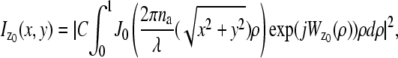 |
(8) |
|---|
where ( denotes an arbitrary point on the detector plane; C is a constant with complex amplitude; λ denotes the wavelength of the detected photons; _n_a denotes the numerical aperture of the objective lens; _J_0 denotes the 0th-order Bessel function of the first kind; and
  ρ ∈ [0, 1], denotes the phase aberration term. We note that Eq. 8 provides a general expression for several 3D PSF models (62), which describes the image of a point-source/single-molecule and is based on scalar diffraction theory. Rewriting Eq. 8 in terms of an image function, we have
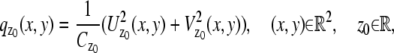 |
(9) |
|---|
where
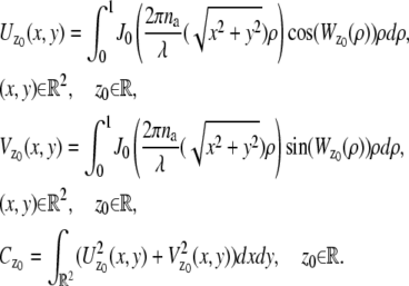 |
(10) |
|---|
In the above equation,  denotes the real (imaginary) part of
  given in Eq. 8. The term
  is the normalization constant, and the
  scaling in Eq. 9 ensures that
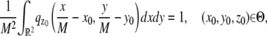
where M denotes the lateral magnification of the objective lens. Although, not shown explicitly, it can be verified that  and the partial derivative of
  with respect to _z_0 are laterally symmetric along the x and y axes with respect to (0, 0), for
To calculate the 3D PSF, we require an explicit analytical expression for the phase aberration term  and here, we set
  to be
to be
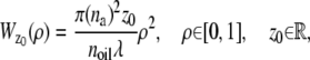 |
(11) |
|---|
where _n_a denotes the numerical aperture of the objective lens, _n_oil denotes the refractive index of the immersion oil, and _z_0 denotes the axial coordinate of the single molecule in the object space.
To calculate Eq. 2 we also require the partial derivatives of  with respect to x, y, and z0, and these are given as
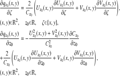
where for ζ ∈ {x, y},
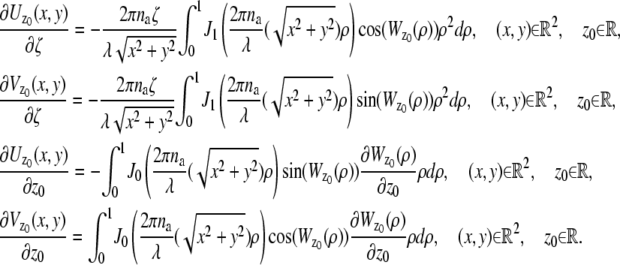
For the MUM setup, the expression for the Fisher information matrix is analogous to that of the conventional microscope and therefore the above expressions for  and their partial derivatives can be used for the calculation of the Fisher information matrix.
Effects of pixelation and extraneous noise sources
We next consider the calculation of the Fisher information matrix that takes into account deteriorating experimental factors. Here, we first consider the multifocal plane microscope setup for which the expression for the Fisher information matrix is given by Eq. 5. For calculating Eq. 5, we require analytical expressions for  and
and  which are given by Eqs. 6 and 7. We also require analytical expressions for the partial derivative of
  j = 1, 2, with respect to the components of θ, and these are given as
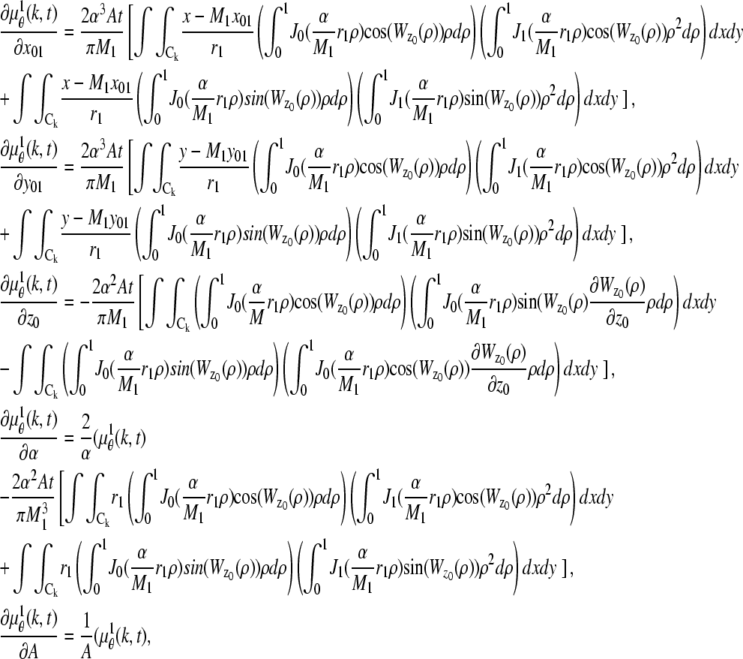
where θ ∈ Θ, k = 1,…,_N_1; α = 2_πn_a/λ;  ρ ∈ [0, 1]; and
  ρ ∈ [0, 1]. The expression for the partial derivative of
  is analogous to that of
  except that in the above equations _M_1 is replaced by _M_2, _x_01 and _y_01 are replaced by _x_02 and _y_02, respectively, _r_1 is replaced by _r_2, where
  _z_0 is replaced by _z_0 – _δz_f, and _N_1 is replaced by _N_2. For a conventional microscope, the analytical expression for μ θ is analogous to Eq. 6 and the expressions for the partial derivative of μ θ, with respect to the components of θ being analogous to the above equations.
To calculate the 3D localization measure, we need to evaluate the above expressions for which we require numerical values of _M_1, _M_2, _x_01, _y_01, _x_02, _y_02, _z_0, α, A, and the background parameters. The calculations for the simulated data are straightforward since the numerical values for all these parameters are known. For experimental data, the magnifications _M_1 and _M_2, and the background parameters are determined as described in Methods.
The numerical values of the 3D localization measure for the fixed cell imaging data reported in Tables 2 and 3 were determined by using the mean value of the estimates of _x_01, _y_01, _x_02, _y_02, _z_0, α, and A for a given focus level. In the case of live-cell imaging data, the range of the 3D localization measure values was calculated by using estimates of _x_01, _y_01, _x_02, _y_02, _z_0, α, and A determined from the QD images in the live cell data.
References
- 1.Kwik, J., S. Boyle, D. Fooksman, L. Margolis, M. P. Sheetz, and M. Edidin. 2003. Membrane cholesterol, lateral mobility, and the phosphatidylinositol 4,5-bisphosphate-dependent organization of cell actin. Proc. Natl. Acad. Sci. USA. 100:13964–13969. [DOI] [PMC free article] [PubMed] [Google Scholar]
- 2.Zenisek, D., J. A. Steyer, and W. Almers. 2000. Transport, capture and exocytosis of single synaptic vesicles at active zones. Nature. 406:849–854. [DOI] [PubMed] [Google Scholar]
- 3.Ehrlich, M., W. Boll, A.Van Oijen, R. Haniharan, K. Chandran, M. L. Nibert, and T. Kirchhausen. 2004. Endocytosis by random initiation and stabilization of clathrin-coated pits. Cell. 118:591–605. [DOI] [PubMed] [Google Scholar]
- 4.Hua, W., D. Sheff, D. Toomre, and I. Mellman. 2006. Vectorial insertion of apical and basolateral membrane proteins in polarized epithelial cells revealed by quantitative 3D live-cell imaging. J. Cell Biol. 172:1035–1044. [DOI] [PMC free article] [PubMed] [Google Scholar]
- 5.Ober, R. J., C. Martinez, X. Lai, J. Zhou, and E. S. Ward. 2004. Exocytosis of IgG as mediated by the receptor, FcRn: an analysis at the single molecule level. Proc. Natl. Acad. Sci. USA. 101:11076–11081. [DOI] [PMC free article] [PubMed] [Google Scholar]
- 6.Oheim, M. 2004. A deeper look into single-secretory vesicle dynamics. Biophys. J. 87:1403–1405. [DOI] [PMC free article] [PubMed] [Google Scholar]
- 7.Rutter, G. A., and E. V. Hill. 2006. Insulin vesicle release: walk, kiss, pause… then run. Physiology (Bethesda). 21:189–196. [DOI] [PubMed] [Google Scholar]
- 8.Conner, S. D., and S. L. Schmid. 2003. Regulated portals of entry into the cell. Nature. 422:37–44. [DOI] [PubMed] [Google Scholar]
- 9.Maxfield, F. R., and T. E. McGraw. 2004. Endocytic recycling. Nat. Rev. Mol. Cell Biol. 5:121–132. [DOI] [PubMed] [Google Scholar]
- 10.Pelkmans, L., and M. Zerial. 2005. Kinase-regulated quantal assemblies and kiss-and-run recycling of caveolae. Nature. 436:128–133. [DOI] [PubMed] [Google Scholar]
- 11.Schütz, G. J., M. Axman, and H. Schindler. 2001. Imaging single molecules in three dimensions. Single Mol. 2:69–74. [Google Scholar]
- 12.Arhel, N., A. Genovesio, K. A. Kim, S. Miko, E. Perret, J. C. Olivo-Marin, S. Shorte, and P. Charneau. 2006. Quantitative four-dimensional tracking of cytoplasmic and nuclear HIV-1 complexes. Nat. Methods. 3:817–824. [DOI] [PubMed] [Google Scholar]
- 13.Thomann, D., D. R. Rines, P. K. Sorger, and G. Danuser. 2002. Automatic fluorescent tag detection in 3D with super-resolution: application to the analysis of chromosome movement. J. Microsc. 208:49–64. [DOI] [PubMed] [Google Scholar]
- 14.Sako, Y., S. Minoghchi, and T. Yanagida. 2000. Single-molecule imaging of EGFR signaling on the surface of living cells. Nat. Cell Biol. 2:168–172. [DOI] [PubMed] [Google Scholar]
- 15.Moerner, W. E. 2007. New directions in single-molecule imaging and analysis. Proc. Natl. Acad. Sci. USA. 104:12596–12602. [DOI] [PMC free article] [PubMed] [Google Scholar]
- 16.Speidel, M., A. Jonas, and E. L. Florin. 2003. Three-dimensional tracking of fluorescent nanoparticles with subnanometer precision by use of off-focus imaging. Opt. Lett. 28:69–71. [DOI] [PubMed] [Google Scholar]
- 17.Toprak, E., H. Balci, B. H. Blehm, and P. R. Selvin. 2007. Three-dimensional particle tracking via bifocal imaging. Nano Lett. 7:2043–2045. [DOI] [PubMed] [Google Scholar]
- 18.Aguet, F., D. V. D. Ville, and M. Unser. 2005. A maximum likelihood formalism for sub-resolution axial localization of fluorescent nanoparticles. Opt. Exp. 13:10503–10522. [DOI] [PubMed] [Google Scholar]
- 19.Kao, H. P., and A. S. Verkman. 1994. Tracking of single fluorescent particles in three dimensions: use of cylindrical optics to encode particle position. Biophys. J. 67:1291–1300. [DOI] [PMC free article] [PubMed] [Google Scholar]
- 20.Holtzer, L., T. Meckel, and T. Schmidt. 2007. Nanometric 3D tracking of individual quantum dots in cells. Appl. Phys. Lett. 90:053902. [Google Scholar]
- 21.Huang, B., W. Wang, M. Bates, and X. Zhuang. 2008. Three-dimensional super-resolution imaging by stochastic optical reconstruction microscopy. Science. 319:810–813. [DOI] [PMC free article] [PubMed] [Google Scholar]
- 22.Watanabe, T. M., and H. Higuchi. 2007. Stepwise movements in vesicle transport of HER2 by motor proteins in living cells. Biophys. J. 92:4109–4120. [DOI] [PMC free article] [PubMed] [Google Scholar]
- 23.Levi, V., Q. Ruan, and E. Gratton. 2005. 3D particle tracking in a two-photon microscope: application to the study of molecular dynamics in cells. Biophys. J. 88:2919–2928. [DOI] [PMC free article] [PubMed] [Google Scholar]
- 24.Dahan, M., S. Levi, C. Luccardini, P. Rostaing, B. Riveau, and A. Triller. 2003. Diffusion dynamics of glycine receptors revealed by single-quantum dot tracking. Science. 302:442–445. [DOI] [PubMed] [Google Scholar]
- 25.Crane, J., and A. Verkman. 2008. Long-range nonanomalous diffusion of quantum dot-labeled aquaporin-1 water channels in the cell plasma membrane. Biophys. J. 94:702–713. [DOI] [PMC free article] [PubMed] [Google Scholar]
- 26.Nan, X., P. A. Sims, P. Chen, and X. S. Xie. 2005. Observation of individual microtubule motor steps in living cells with endocytosed quantum dots. J. Phys. Chem. B. 109:24220–24224. [DOI] [PubMed] [Google Scholar]
- 27.Courty, S., C. Luccardini, Y. Bellaiche, G. Cappello, and M. Dahan. 2006. Tracking individual kinesin motors in living cells using single quantum-dot imaging. Nano Lett. 6:1491–1495. [DOI] [PubMed] [Google Scholar]
- 28.Cui, B., C. Wu, L. Chen, A. Ramirez, E. L. Bearer, W. Li, W. C. Mobley, and S. Chu. 2007. One at a time, live tracking of NGF axonal transport using quantum dots. Proc. Natl. Acad. Sci. USA. 104:13666–13671. [DOI] [PMC free article] [PubMed] [Google Scholar]
- 29.Lidke, K. A., B. Rieger, T. M. Jovin, and R. Heintzmann. 2005. Superresolution by localization of quantum dots using blinking statistics. Opt. Exp. 13:7052–7062. [DOI] [PubMed] [Google Scholar]
- 30.Rust, M., M. Bates, and X. Zhuang. 2006. Sub-diffraction-limit imaging by stochastic optical reconstruction microscopy (STORM). Nat. Methods. 3:793–795. [DOI] [PMC free article] [PubMed] [Google Scholar]
- 31.Betzig, E., G. H. Patterson, R. Sougrat, O. W. Lindwasser, S. Olenych, J. S. Bonifacino, M. W. Davidson, J. Lippincott-Schwartz, and H. F. Hess. 2006. Imaging intracellular fluorescent proteins at nanometer resolution. Science. 313:1642–1645. [DOI] [PubMed] [Google Scholar]
- 32.Hess, S. T., T. P. K. Girirajan, and M. D. Mason. 2006. Ultra-high resolution imaging by fluorescence photoactivation localization microscopy. Biophys. J. 91:4258–4272. [DOI] [PMC free article] [PubMed] [Google Scholar]
- 33.Egner, A., C. Geisler, C. V. Middendorff, H. Bock, D. Wenzel, R. Medda, M. Andresen, A. C. Stiel, S. Jakobs, C. Eggeling, A. Schonle, and S. Hell. 2007. Fluorescence nanoscopy in whole cells by asynchronous localization of photoswitching emitters. Biophys. J. 93:3285–3290. [DOI] [PMC free article] [PubMed] [Google Scholar]
- 34.Ober, R. J., S. Ram, and E. S. Ward. 2004. Localization accuracy in single molecule microscopy. Biophys. J. 86:1185–1200. [DOI] [PMC free article] [PubMed] [Google Scholar]
- 35.Thompson, R. E., D. R. Larson, and W. W. Webb. 2002. Precise nanometer localization analysis for individual fluorescent probes. Biophys. J. 82:2775–2783. [DOI] [PMC free article] [PubMed] [Google Scholar]
- 36.Folling, J., V. Belov, R. Kunetsky, R. Medda, A. Schonle, A. Egner, C. Eggeling, M. Bossi, and S. W. Hell. 2007. Photochromic rhodamines provide nanoscopy with optical sectioning. Angew. Chem. 46:6266–6270. [DOI] [PubMed] [Google Scholar]
- 37.Juette, M. F., T. J. Gould, M. D. Lessard, M. J. Mlodzianoski, B. Nagpure, B. T. Bennett, S. T. Hess, and J. Bewersdorf. 2008. Three-dimensional sub-100 nm resolution fluorescence microscopy of thick samples. Nat. Methods. 5:527–529. [DOI] [PubMed] [Google Scholar]
- 38.Hess, S. T., T. J. Gould, M. V. Gudheti, S. A. Maas, K. D. Mills, and J. Zimmerberg. 2007. Dynamic clustered distribution of hemagglutinin resolved at 40 nm in living cell membranes discriminates between raft theories. Proc. Natl. Acad. Sci. USA. 104:17370–17375. [DOI] [PMC free article] [PubMed] [Google Scholar]
- 39.Manley, S., J. M. Gillette, G. H. Patterson, H. Shroff, H. F. Hess, E. Betzig, and J. Lippincott-Schwartz. 2008. High-density mapping of single-molecule trajectories with photoactivated localization microscopy. Nat. Methods. 5:155–157. [DOI] [PubMed] [Google Scholar]
- 40.Shroff, H., C. G. Galbraith, J. A. Galbraith, and E. Betzig. 2008. Live-cell photoactivated localization microscopy of nanoscale adhesion dynamics. Nat. Methods. 5:417–423. [DOI] [PMC free article] [PubMed] [Google Scholar]
- 41.Prabhat, P., S. Ram, E. S. Ward, and R. J. Ober. 2004. Simultaneous imaging of different focal planes in fluorescence microscopy for the study of cellular dynamics in three dimensions. IEEE Trans. Nanobioscience. 3:237–242. [DOI] [PMC free article] [PubMed] [Google Scholar]
- 42.Prabhat, P., Z. Gan, J. Chao, S. Ram, C. Vaccaro, S. Gibbons, R. J. Ober, and E. S. Ward. 2007. Elucidation of intracellular pathways leading to exocytosis of the Fc receptor, FcRn, using multifocal plane microscopy. Proc. Natl. Acad. Sci. USA. 104:5889–5894. [DOI] [PMC free article] [PubMed] [Google Scholar]
- 43.Ghetie, V., and E. S. Ward. 2000. Multiple roles for the major histocompatibility complex class I-related receptor FcRn. Annu. Rev. Immunol. 18:739–766. [DOI] [PubMed] [Google Scholar]
- 44.Ram, S., E. S. Ward, and R. J. Ober. 2006. A stochastic analysis of performance limits for optical microscopes. Multidim. Sys. Sig. Proc. 17:27–58. [Google Scholar]
- 45.Rao, C. R. 1965. Linear Statistical Inference and its Applications. Wiley, New York.
- 46.Snyder, D. L., and M. I. Miller. 1991. Random Point Processes in Time and Space, 2nd Ed. Springer Verlag, New York.
- 47.Ram, S., E. S. Ward, and R. J. Ober. 2005. How accurately can a single molecule be localized in three dimensions using a fluorescence microscope? Proc. SPIE. 5699:426–435. [DOI] [PMC free article] [PubMed] [Google Scholar]
- 48.Gibson, S. F., and F. Lanni. 1989. Diffraction by a circular aperture as a model for 3D optical microscopy. J. Opt. Soc. Am. A. 6:1357–1367. [DOI] [PubMed] [Google Scholar]
- 49.Ram, S., J. Chao, P. Prabhat, E. S. Ward, and R. J. Ober. 2007. A novel approach to determining the 3D location of microscopic objects with applications to 3D particle tracking. Proc. SPIE. 6443:D1–D7. [Google Scholar]
- 50.Microscopy Image Analysis Tool (MIATool) software package. Ward Lab, Southwestern Medical Center, Dallas, TX. http://www4.utsouthwestern.edu/wardlab/miatool.
- 51.Saxton, M. J., and K. Jacobson. 1997. Single particle tracking: applications to membrane dynamics. Annu. Rev. Biophys. Biomol. Struct. 26:373–399. [DOI] [PubMed] [Google Scholar]
- 52.Ades, E. W., F. J. Candal, R. A. Swerlick, V. G. George, S. Summers, D. C. Bosse, and T. J. Lawley. 1992. HMEC-1: establishment of an immortalized human microvascular endothelial cell line. J. Invest. Dermatol. 99:683–690. [DOI] [PubMed] [Google Scholar]
- 53.Ober, R. J., C. Martinez, C. Vaccaro, J. Zhou, and E. S. Ward. 2004. The site and dynamics of IgG salvage by the MHC class I-related receptor, FcRn. J. Immunol. 172:2021–2029. [DOI] [PubMed] [Google Scholar]
- 54.Zhou, Z., F. Mateos, R. J. Ober, and E. S. Ward. 2005. Conferring the binding properties of the mouse MHC class-I related receptor, FcRn, onto the human ortholog by sequential rounds of site-directed mutagenesis. J. Mol. Biol. 345:1071–1081. [DOI] [PubMed] [Google Scholar]
- 55.Cheezum, M. K., W. F. Walker, and W. H. Guilford. 2001. Quantitative comparison of algorithms for tracking single fluorescent particles. Biophys. J. 81:2378–2388. [DOI] [PMC free article] [PubMed] [Google Scholar]
- 56.Carter, P. J. 2006. Potent antibody therapeutics by design. Nat. Rev. Immunol. 6:343–357. [DOI] [PubMed] [Google Scholar]
- 57.Smith, P. R., I. E. G. Morrison, K. M. Wilson, N. Fernandez, and R. J. Cherry. 1999. Anomalous diffusion of major histocompatibility complex class-I molecules on HeLa cells determined by single particle tracking. Biophys. J. 76:3331–3344. [DOI] [PMC free article] [PubMed] [Google Scholar]
- 58.Iino, R., I. Koyama, and A. Kusumi. 2001. Single molecule imaging of green fluorescent proteins in living cells: E-cadherin forms oligomers on the free cell surface. Biophys. J. 80:2667–2677. [DOI] [PMC free article] [PubMed] [Google Scholar]
- 59.Capps, G. G., S. Pine, M. Edidin, and M. C. Zuniga. 2004. Short class I major histocompatibility complex cytoplasmic tails differing in charge detect arbiters of lateral diffusion in the plasma membrane. Biophys. J. 86:2896–2909. [DOI] [PMC free article] [PubMed] [Google Scholar]
- 60.King, S. J., and T. A. Schroer. 2000. Dynactin increases the processivity of the cytoplasmic dynein motor. Nat. Cell Biol. 2:20–24. [DOI] [PubMed] [Google Scholar]
- 61.Lidke, D. S., P. Nagy, and D. J. Arndt-Jovin. 2007. In vivo imaging using quantum dot-conjugated probes. Curr. Protoc. Cell Biol. 25:1–18. [DOI] [PubMed] [Google Scholar]
- 62.Gibson, S. F. 1990. Modeling the 3D imaging properties of the fluorescence light microscope. PhD thesis, Carnegie-Mellon University, Pittsburgh, PA.
Associated Data
This section collects any data citations, data availability statements, or supplementary materials included in this article.
Supplementary Materials
[Supplement]