Model-based analysis of oligonucleotide arrays: model validation, design issues and standard error application - PubMed (original) (raw)
Model-based analysis of oligonucleotide arrays: model validation, design issues and standard error application
C Li et al. Genome Biol. 2001.
Abstract
Background: A model-based analysis of oligonucleotide expression arrays we developed previously uses a probe-sensitivity index to capture the response characteristic of a specific probe pair and calculates model-based expression indexes (MBEI). MBEI has standard error attached to it as a measure of accuracy. Here we investigate the stability of the probe-sensitivity index across different tissue types, the reproducibility of results in replicate experiments, and the use of MBEI in perfect match (PM)-only arrays.
Results: Probe-sensitivity indexes are stable across tissue types. The target gene's presence in many arrays of an array set allows the probe-sensitivity index to be estimated accurately. We extended the model to obtain expression values for PM-only arrays, and found that the 20-probe PM-only model is comparable to the 10-probe PM/MM difference model, in terms of the expression correlations with the original 20-probe PM/MM difference model. MBEI method is able to extend the reliable detection limit of expression to a lower mRNA concentration. The standard errors of MBEI can be used to construct confidence intervals of fold changes, and the lower confidence bound of fold change is a better ranking statistic for filtering genes. We can assign reliability indexes for genes in a specific cluster of interest in hierarchical clustering by resampling clustering trees. A software dChip implementing many of these analysis methods is made available.
Conclusions: The model-based approach reduces the variability of low expression estimates, and provides a natural method of calculating expression values for PM-only arrays. The standard errors attached to expression values can be used to assess the reliability of downstream analysis.
Figures
Figure 1
values for probe sets. values estimated for probe sets (a) 6457, (b) 1248, and (c) 6571 in six array sets (shown in panels 1–6 from left to right for each probe set). values (constrained to have sum square equal to number of probes used in each array set) are on the _y_-axis, and probe pairs are labeled 1 to 20 on the _x_-axis. The title of each panel (for example, p = 0) indicates the proportion of arrays 'present' for the target gene in the array set. Large circles represent identified probe-outliers by negativity or large SE of .
Figure 2
Boxplots of average pairwise correlations of
s between two array sets. They are stratified by average lower presence proportion in two array sets (the presence proportion of a probe set is the proportion of arrays in an array set where the target gene is called 'present' by GeneChip's algorithm). The average is taken over C(6, 2) = 15 pairwise comparison of two array sets for each probe set, and the correlation is calculated using probes that are not identified as an outlier in both array sets. The range of the average lower presence proportion for the six boxplots are: (0, 0.17), (0.17, 0.34), (0.34, 0.51), (0.51, 0.68), (0.68, 0.85), (0.85, 1). The title of each boxplot is the number of probe sets classified into this boxplot. Eleven probe sets with too few non-outlier probes to calculate correlations for all 15 comparisons are not included in the boxplots. The average lower presence proportion and average pairwise correlation for probe sets in Figure 1 are (a) 1, 0.95; (b), 0.93, 0.94; and (c) 0, 0.86.
Figure 3
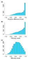
Histogram of correlations between model-based expression values estimated using the 20-probe difference model and those estimated using different models. (a) 10-probe difference model; (b) 20-probe PM-only model; (c) 20-probe MM-only model. All comparisons are across the 21 arrays in array set 1.
Figure 4
Boxplot of correlations between θ values estimated using the 20-probe difference model and θs estimated using different models, stratified by presence proportion. (a) 10-probe difference model; (b) 20-probe PM-only model; and (c) 20-probe MM-only model. The number of presence calls for a probe set in the 21 arrays and the subpopulation size for the six boxplots are: 0–3, 4,385; 4–7, 693; 8–11, 413; 12–15, 488; 16–19, 497; and 20–21, 323. Only 6,799 probe sets that have 20 probes are used.
Figure 5
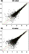
Log (base 10) expression indexes of a pair of replicate arrays (array 1 and 2 of array set 5) for different statistical methods. (a) MBEI method; (b) AD method. Only 6,695 (a) and 4,696 (b) probe sets with positive values in both arrays are used. The center line is y = x, and the flanking lines indicate the difference of a factor of two.
Figure 6
Boxplots of average absolute log (base 10) ratios between replicate arrays stratified by presence proportion for different statistical methods. (a) MBEI method; (b) AD method. The number of presence calls for a probe set in the 58 arrays for the six boxplots are: 0–9, 10–19, 20–29, 30–39, 40–49, 50–58. The title of each boxplot is the number of probe sets used for the boxplot. The average is taken over 29 replicate pairs. Log ratios are not calculated for negative expression values or expression values identified as 'array-outliers' by the MBEI method in either array of a replicate pair, and are not used to calculate the average. 744 probe sets are not included as their average absolute log ratios cannot be calculated for all the 29 pairs using either method.
Figure 7
Similar plots as in Figure 6 for another set of 30 pairs of duplicated human U95A arrays. (a) MBEI method; (b) AD method.The number of presence calls for a probe set in the 60 arrays for the six boxplots are: 0–9, 10–19, 20–29, 30–39, 40–49, 50–60. The title of each boxplot is the number of probe sets used for the boxplot.
Figure 8
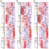
Gene clustering (a) 225 filtered genes are clustered based on their expression profiles across 20 samples. Each gene's expression values are standardized to have mean 0 and SD 1 across 20 samples. Dark blue represents low expression level and dark red high expression level. We might be particularly interested in the cluster colored in blue. (b) The clustering tree after a particular resampling. Although the original 'blue' genes are scattered to various places, we can still determine where the original cluster is, using the criteria described in the text. (c) After resampling 30 times, the reliability of the genes belonging to the original cluster is indicated by the vertical gray-scale bar on the left of the blue-red picture.
Figure 9
Normalization of gene expression levels between arrays. (a) The CEL intensities (see text) of a pair of replicate arrays (array 11 and 12 in array set 5) are plotted against each other. The baseline array 11 (shown on the _y_-axis) is not as bright as array 12 (shown on the _x_-axis). The smoothing spline (green curve) deviates from the diagonal line y = x (blue curve), indicating the need for normalization. (b) The same plot as (a) with superimposed circles representing the invariant set, on the basis of which a piecewise linear normalization relationship is determined (black dotted line, whose _y_-coordinate is the normalized value of array 12). The normalization curve is close to the smoothing spline curve in (a) as the two arrays are replicated arrays and all probes should be invariant. (c) After normalization (_y_-axis is the baseline array 11, and _x_-axis the normalized value of array 12), the scatterplot centers around the diagonal line and the array 12 is adjusted to have the similar overall brightness as array 11. The smoothing spline curve is also close to the diagonal line. (d) The Q-Q plot of probe intensities of array 11 and normalized array 12 shows the probes in the two sets have almost the same distribution.
Figure 10
Similar plots as in Figure 9 for arrays hybridized to two different samples (array 24 and 36 of array set 5). (a) CEL intensities; (b) same plot as in (a) with superimposed circles representing the invariant set; (c) after renormalization; (d) Q-Q plot of normalized probe intensities. Note that the smoothing spline in (a) is affected by several points at the lower-right corner, which might belong to differentially expressed genes. The invariant set, on the other hand, does not include these points when determining the normalization curve, leading to a different normalization relationship at the high end.
Similar articles
- Theoretical and experimental comparisons of gene expression indexes for oligonucleotide arrays.
Lemon WJ, Palatini JJ, Krahe R, Wright FA. Lemon WJ, et al. Bioinformatics. 2002 Nov;18(11):1470-6. doi: 10.1093/bioinformatics/18.11.1470. Bioinformatics. 2002. PMID: 12424118 - Exploration, normalization, and summaries of high density oligonucleotide array probe level data.
Irizarry RA, Hobbs B, Collin F, Beazer-Barclay YD, Antonellis KJ, Scherf U, Speed TP. Irizarry RA, et al. Biostatistics. 2003 Apr;4(2):249-64. doi: 10.1093/biostatistics/4.2.249. Biostatistics. 2003. PMID: 12925520 - Statistical analysis of high-density oligonucleotide arrays: a multiplicative noise model.
Sásik R, Calvo E, Corbeil J. Sásik R, et al. Bioinformatics. 2002 Dec;18(12):1633-40. doi: 10.1093/bioinformatics/18.12.1633. Bioinformatics. 2002. PMID: 12490448 - Fundamentals of DNA hybridization arrays for gene expression analysis.
Freeman WM, Robertson DJ, Vrana KE. Freeman WM, et al. Biotechniques. 2000 Nov;29(5):1042-6, 1048-55. doi: 10.2144/00295rv01. Biotechniques. 2000. PMID: 11084867 Review. - Post-analysis follow-up and validation of microarray experiments.
Chuaqui RF, Bonner RF, Best CJ, Gillespie JW, Flaig MJ, Hewitt SM, Phillips JL, Krizman DB, Tangrea MA, Ahram M, Linehan WM, Knezevic V, Emmert-Buck MR. Chuaqui RF, et al. Nat Genet. 2002 Dec;32 Suppl:509-14. doi: 10.1038/ng1034. Nat Genet. 2002. PMID: 12454646 Review.
Cited by
- Gene expression microarray analysis of the spinal trigeminal nucleus in a rat model of migraine with aura.
Liu R, Yu S, Li F, Qiu E. Liu R, et al. Neural Regen Res. 2012 Sep 5;7(25):1931-8. doi: 10.3969/j.issn.1673-5374.2012.25.002. Neural Regen Res. 2012. PMID: 25624821 Free PMC article. - Expression-based and co-localization detection of arabinogalactan protein 6 and arabinogalactan protein 11 interactors in Arabidopsis pollen and pollen tubes.
Costa M, Nobre MS, Becker JD, Masiero S, Amorim MI, Pereira LG, Coimbra S. Costa M, et al. BMC Plant Biol. 2013 Jan 8;13:7. doi: 10.1186/1471-2229-13-7. BMC Plant Biol. 2013. PMID: 23297674 Free PMC article. - Localization, morphology and transcriptional profile of Aspergillus flavus during seed colonization.
Dolezal AL, Obrian GR, Nielsen DM, Woloshuk CP, Boston RS, Payne GA. Dolezal AL, et al. Mol Plant Pathol. 2013 Dec;14(9):898-909. doi: 10.1111/mpp.12056. Epub 2013 Jul 8. Mol Plant Pathol. 2013. PMID: 23834374 Free PMC article. - PAIR: paired allelic log-intensity-ratio-based normalization method for SNP-CGH arrays.
Yang S, Pounds S, Zhang K, Fang Z. Yang S, et al. Bioinformatics. 2013 Feb 1;29(3):299-307. doi: 10.1093/bioinformatics/bts683. Epub 2012 Nov 29. Bioinformatics. 2013. PMID: 23196989 Free PMC article. - Host response signature to Staphylococcus aureus alpha-hemolysin implicates pulmonary Th17 response.
Frank KM, Zhou T, Moreno-Vinasco L, Hollett B, Garcia JG, Bubeck Wardenburg J. Frank KM, et al. Infect Immun. 2012 Sep;80(9):3161-9. doi: 10.1128/IAI.00191-12. Epub 2012 Jun 25. Infect Immun. 2012. PMID: 22733574 Free PMC article.
References
- Wodicka L, Dong H, Mittmann M, Ho M, Lockhart D. Genome-wide expression monitoring in Saccharomyces cerevisiae. Nat Biotechnol. 1997;15:1359–1367. - PubMed
- Wallace D. The Behrens-Fisher and Fieller-Creasy problems. In Lecture Notes in Statistics 1, RAFisher: An Appreciation Edited by Fienberg SE, Hinkley DV Springer-Verlag. 1988. pp. 119–147.
- Cox DR, Hinkley DV. Theoretical Statistics London: Chapman and Hall, 1974.
Publication types
MeSH terms
Substances
LinkOut - more resources
Full Text Sources
Other Literature Sources


