Normalization using weighted negative second order exponential error functions (NeONORM) provides robustness against asymmetries in comparative transcriptome profiles and avoids false calls - PubMed (original) (raw)
Comparative Study
Normalization using weighted negative second order exponential error functions (NeONORM) provides robustness against asymmetries in comparative transcriptome profiles and avoids false calls
Sebastian Noth et al. Genomics Proteomics Bioinformatics. 2006 May.
Abstract
Studies on high-throughput global gene expression using microarray technology have generated ever larger amounts of systematic transcriptome data. A major challenge in exploiting these heterogeneous datasets is how to normalize the expression profiles by inter-assay methods. Different non-linear and linear normalization methods have been developed, which essentially rely on the hypothesis that the true or perceived logarithmic fold-change distributions between two different assays are symmetric in nature. However, asymmetric gene expression changes are frequently observed, leading to suboptimal normalization results and in consequence potentially to thousands of false calls. Therefore, we have specifically investigated asymmetric comparative transcriptome profiles and developed the normalization using weighted negative second order exponential error functions (NeONORM) for robust and global inter-assay normalization. NeONORM efficiently damps true gene regulatory events in order to minimize their misleading impact on the normalization process. We evaluated NeONORM's applicability using artificial and true experimental datasets, both of which demonstrated that NeONORM could be systematically applied to inter-assay and inter-condition comparisons.
Figures
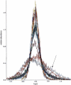
Fig. 1
Asymmetric heavy tails in fold-change distributions. A histogram view of nine different “real-world” superimposed fold-change distributions is shown as calculated from recent experimental work in our laboratory. The arrow indicates asymmetric heavy tails that are observed to different degrees in such experimental data.
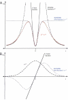
Fig. 2
The NeONORM error function. A. Schematic representation of the standard quadratic error function (solid black), as well as a damping function (dashed black), the product of both (dashed red), and the novel NeONORM error function (dashed blue) that we indirectly derived from the former. B. NeONORM damping function (dashed black) for the first derivative of the NeONORM error function, and the first derivate of the standard quadratic (solid black) and NeONORM (dashed blue) error functions.
Fig. 3
Properties of the NeONORM error function. The NeONORM (composite) error function has exactly one minimum for τ ≤ 2 in the limit of identical weights for both individual error functions. Thereby τ denotes the absolute distance between the global minima of the individual error functions in units of k. Here k is the NeONORM sensitivity parameter identical to the absolute distance between the inclination points and the global minimum of each function. In the upper panel, we schematize the derivatives of the individual NeONORM contributing error functions (black: probe 1, blue: probe 2), and their composite (red) for different values of τ at constant k (shown are the first order derivates in the normalization factor a). The lower panel displays the original functions. Only when τ increases above 2, the NeONORM error function acquires two distinct minima.
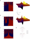
Fig. 4
The NeONORM sensitivity parameter k. A. Sign plot and 3D-surface plot for the first order derivative in a of the NeONORM error as a function of the sensitivity parameter k and the normalization factor a. Sign plots are used to illustrate the zero crossings of the function (blue-red and red-blue boundaries). The data represented are a subtraction from two HT29 technical replicates HT29(1) vs. HT29(2). B. As in panel A for a subtraction between the modified, artificial dataset HT29(1)mod 14 1.5±0.15 vs. HT29(2). In order to generate the modified dataset, a random chosen quarter of all probe signals of the HT29(1) dataset was individually multiplied with a different random value drawn from a normal distribution with _μ_=21.5 and _σ_=0.1*μ. C. As in panel A, but only a sign plot for the second order derivative in a is shown. D. The NeONORM error function for selected increasing values for k is shown for the HT29(1) vs. HT29(2) (upper) and the HT29(1)mod 14 1.5±0.15 vs. HT29(2) datasets. Note that _k_=0.02 is the flattest curve in both cases.
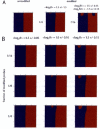
Fig. 5
Artificial “asymmetric” datasets. Sign plots of the NeONORM error function for the first series of artificial test data generated are shown (see Materials and Methods). A. From left to right: (1) Unmodified (original) dataset HT29(1) vs. HT29(2). (2) Asymmetrically modified dataset HT29(1) 14 1.5±1.5 (random chosen quarter, _μ_=21.5 and σ = μ). (3) Double modified dataset HT29(1) 14 1.5±0.15 was once more modified by subsequently choosing another random quarter of probe signals and multiplying them with a random value drawn from a normal distribution with _μ_=2−1.5 and _σ_=0.1*μ. This second operation generates almost symmetrically modified data, where the average total of modified probe signals is 7/16. B. As in panel A. To the right of each row the fraction of modified probe signals (1/16, 1/8, 1/4), and on the top of each column the average ratio change parameters (log2 of μ and the corresponding σ) are indicated.
Fig. 6
The pseudo-code for the implementation of the NeONORM algorithm. Additional details for the implementation can be made available upon written inquiry to the authors.
Fig. 7
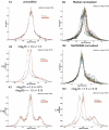
Comparison of Median vs. NeONORM normalization. A. Direct comparison of Median vs. NeONORM on the datasets from Figure 5A. Frequency plots of logQ are shown simultaneously for both methods (Median in grey, NeONORM in red). B. Direct comparison of Median vs. NeONORM on the datasets from Figure 5B. Frequency plots of logQ are shown in the upper two panels simultaneously for all nine datasets (B1: Median normalized, B2: NeONORM normalized). B3: Frequency plots of logQ are shown simultaneously for both methods (Median in grey, NeONORM in red) on the HT29(1)mod 14 1.5±0.15 vs. HT29(2) dataset.
Fig. 8
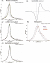
Comparison of Median, LOWESS, and NeONORM normalization. A. Direct comparison of Median, LOWESS, and NeONORM normalization on the artificial datasets summarized in Table 1. Histogram plots of logQ are shown in the three panels simultaneously for all the six modified datasets and the original dataset. B. Direct comparison of Median, LOWESS, and NeONORM normalization on the “real world” NB4 RA 4h vs. NB4 dataset. B1: the first order derivative in a of the NeONORM error function at _k_=0.20, for the range −2 < a < 2. B2: Normalization of the NB4 RA 4h vs. NB4 according to all the three methods (Histogram plot is shown, blue = Median, grey = LOWESS, red = NeONORM).
References
- Stoughton R.B. Applications of DNA microarrays in biology. Annu. Rev. Biochem. 2005;74:53–82. - PubMed
- Raetz E.A., Moos P.J. Impact of microarray technology in clinical oncology. Cancer Invest. 2004;22:312–320. - PubMed
- van Steensel B. Mapping of genetic and epigenetic regulatory networks using microarrays. Nat. Genet. 2005;37:S18–S24. - PubMed
Publication types
MeSH terms
LinkOut - more resources
Full Text Sources
