Mapping trait loci by use of inferred ancestral recombination graphs - PubMed (original) (raw)
Mapping trait loci by use of inferred ancestral recombination graphs
Mark J Minichiello et al. Am J Hum Genet. 2006 Nov.
Abstract
Large-scale association studies are being undertaken with the hope of uncovering the genetic determinants of complex disease. We describe a computationally efficient method for inferring genealogies from population genotype data and show how these genealogies can be used to fine map disease loci and interpret association signals. These genealogies take the form of the ancestral recombination graph (ARG). The ARG defines a genealogical tree for each locus, and, as one moves along the chromosome, the topologies of consecutive trees shift according to the impact of historical recombination events. There are two stages to our analysis. First, we infer plausible ARGs, using a heuristic algorithm, which can handle unphased and missing data and is fast enough to be applied to large-scale studies. Second, we test the genealogical tree at each locus for a clustering of the disease cases beneath a branch, suggesting that a causative mutation occurred on that branch. Since the true ARG is unknown, we average this analysis over an ensemble of inferred ARGs. We have characterized the performance of our method across a wide range of simulated disease models. Compared with simpler tests, our method gives increased accuracy in positioning untyped causative loci and can also be used to estimate the frequencies of untyped causative alleles. We have applied our method to Ueda et al.'s association study of CTLA4 and Graves disease, showing how it can be used to dissect the association signal, giving potentially interesting results of allelic heterogeneity and interaction. Similar approaches analyzing an ensemble of ARGs inferred using our method may be applicable to many other problems of inference from population genotype data.
Figures
Figure 1.
The ARG. A, Example ARG for four chromosome sequences. The sequences label the leaves of the ARG and are written as strings of 0s and 1s (coding SNP alleles). Moving backward in time (up the ARG), one first encounters a mutation. A mutation is denoted by a black dot and a number specifying its marker position. The second event is a recombination between markers 2 and 3. As one works backward in time, this corresponds to splitting a lineage into two, with the alleles at positions 1 and 2 following the left lineage and the allele at position 3 following the right lineage. After this is a coalescence, merging two lineages into one, and so on, to the grand common ancestor. B, Marginal tree for the SNPs at positions 1 and 2. C, Marginal tree for the SNP at position 3. To test a marginal tree for disease association, mutations are dropped onto each of the branches in turn, defining hypothetical allelic states of the leaves, which can then be tested for statistical association with the phenotype. The black dot labeled “2” best segregates the cases (D) from the controls (U) and would be identified as the most likely causative mutation event. D–G, Logic behind the ARG inference algorithm. D, The two sequences have a shared tract over the region . E, To coalesce over the tract region, we must add a recombination breakpoint to the right of it—that is, between positions 2 and 3. This results in two parent sequences. F, We let undefined material (denoted by
·
) coalesce with anything. We can now coalesce the left recombination parent and the other sequence. G, We can add a mutation.
Figure 2.
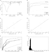
Analysis of a suite of case-control studies with disease parameters
GRR(Aa)=2
,
GRR(AA)=3
,
_q_=0.04
, and
n _cc_=2,000
, sampled from the constant population with the full ascertainment tSNP set. A, Association structure for a simulated case-control study.
▵
denotes the position of the (untyped) causative SNP. _B,_Probability of there being a significant association within an interval around the causative SNP. C and D, Markerwise P values at the marker closest to the causative SNP for each of the 50 studies. E, Cumulative distribution of distances between the association peak and the causative SNP. F, Distribution of estimated allele frequency.
Figure 3.
Marginal tree correlation versus
_r_2
LD for part of ENCODE region 7p15.2 from the phase I HapMap. Tree correlation is measured as the proportion of the
_n_-3
nonequivalent, nonunary bipartitions of the leaves of each tree (defined by cutting branches) that are shared between trees at different positions.
Figure 4.
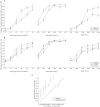
Power, localization, and interpretation for a range of disease models. Each point on the _X_-axis corresponds to a suite of 50 studies. Each of the disease parameters is varied between suites, whereas the other parameters are held at “default” values of
GRR(Aa)=2
,
GRR(AA)=2×GRR(Aa)-1
,
_q_=0.04
, and
n _cc_=2,000
. All studies are sampled from the constant population with the full ascertainment tSNP set. A, Probability of an experimentwise significant signal within 100 kb of the causative SNP (calculated as the proportion of studies in each suite that meet this criterion). B, Probability that the association peak is within 100 kb of the causative SNP. C, Estimated causative-allele frequency versus true frequency q.
Figure 5.
Localization for different data, populations, and tSNP models. A, Performance on a suite of case-control studies with
GRR(Aa)=2
,
GRR(AA)=3
,
_q_=0.04
, and
n _cc_=2,000
, sampled from the constant population and with the full ascertainment tSNP set. Margarita is applied to this suite under three scenarios: when the data are phased, when they are unphased, and when they are phased but have 10% missing data. B, Performance on a suite of case-control studies sampled from the hot population (and with
GRR(Aa)=2
,
GRR(AA)=3
,
_q_=0.04
, and
n _cc_=2,000
). Performance is compared using three different tSNP ascertainment schemes (described in the “Methods” section).
Figure 6.
Analysis of the CTLA4 data. A, Association structure of the region. B, Distribution of estimated causative-allele frequency, by use of marginal trees at CT60. C, Test for allelic heterogeneity, by calculation of the proportion of inferred marginal trees at each position for which a chromosome appears under the branch that best segregates the cases and controls. D, Association structure for a subset of the CTLA4 data—only those chromosomes with the protective CT60 allele.
Similar articles
- The Promise of Inferring the Past Using the Ancestral Recombination Graph.
Brandt DYC, Huber CD, Chiang CWK, Ortega-Del Vecchyo D. Brandt DYC, et al. Genome Biol Evol. 2024 Feb 1;16(2):evae005. doi: 10.1093/gbe/evae005. Genome Biol Evol. 2024. PMID: 38242694 Free PMC article. - tstrait: a quantitative trait simulator for ancestral recombination graphs.
Tagami D, Bisschop G, Kelleher J. Tagami D, et al. Bioinformatics. 2024 Jun 3;40(6):btae334. doi: 10.1093/bioinformatics/btae334. Bioinformatics. 2024. PMID: 38796683 - Coalescent-based association mapping and fine mapping of complex trait loci.
Zöllner S, Pritchard JK. Zöllner S, et al. Genetics. 2005 Feb;169(2):1071-92. doi: 10.1534/genetics.104.031799. Epub 2004 Oct 16. Genetics. 2005. PMID: 15489534 Free PMC article. - The era of the ARG: An introduction to ancestral recombination graphs and their significance in empirical evolutionary genomics.
Lewanski AL, Grundler MC, Bradburd GS. Lewanski AL, et al. PLoS Genet. 2024 Jan 18;20(1):e1011110. doi: 10.1371/journal.pgen.1011110. eCollection 2024 Jan. PLoS Genet. 2024. PMID: 38236805 Free PMC article. Review. - On selecting markers for association studies: patterns of linkage disequilibrium between two and three diallelic loci.
Garner C, Slatkin M. Garner C, et al. Genet Epidemiol. 2003 Jan;24(1):57-67. doi: 10.1002/gepi.10217. Genet Epidemiol. 2003. PMID: 12508256 Review.
Cited by
- Extremely sparse models of linkage disequilibrium in ancestrally diverse association studies.
Salehi Nowbandegani P, Wohns AW, Ballard JL, Lander ES, Bloemendal A, Neale BM, O'Connor LJ. Salehi Nowbandegani P, et al. Nat Genet. 2023 Sep;55(9):1494-1502. doi: 10.1038/s41588-023-01487-8. Epub 2023 Aug 28. Nat Genet. 2023. PMID: 37640881 - A fast algorithm for genome-wide haplotype pattern mining.
Besenbacher S, Pedersen CN, Mailund T. Besenbacher S, et al. BMC Bioinformatics. 2009 Jan 30;10 Suppl 1(Suppl 1):S74. doi: 10.1186/1471-2105-10-S1-S74. BMC Bioinformatics. 2009. PMID: 19208179 Free PMC article. - New Genetic Approaches to AD: Lessons from APOE-TOMM40 Phylogenetics.
Lutz MW, Crenshaw D, Welsh-Bohmer KA, Burns DK, Roses AD. Lutz MW, et al. Curr Neurol Neurosci Rep. 2016 May;16(5):48. doi: 10.1007/s11910-016-0643-8. Curr Neurol Neurosci Rep. 2016. PMID: 27039903 Review. - Multipoint identity-by-descent prediction using dense markers to map quantitative trait loci and estimate effective population size.
Meuwissen TH, Goddard ME. Meuwissen TH, et al. Genetics. 2007 Aug;176(4):2551-60. doi: 10.1534/genetics.107.070953. Epub 2007 Jun 11. Genetics. 2007. PMID: 17565953 Free PMC article. - Identification of copy number variation hotspots in human populations.
Fu W, Zhang F, Wang Y, Gu X, Jin L. Fu W, et al. Am J Hum Genet. 2010 Oct 8;87(4):494-504. doi: 10.1016/j.ajhg.2010.09.006. Am J Hum Genet. 2010. PMID: 20920665 Free PMC article.
References
Web Resources
- BARGEN, http://www.ebi.ac.uk/projects/BARGEN (for downloading the FREGENE simulator)
- Margarita, http://www.sanger.ac.uk/Software/analysis/margarita (for downloading the Java program Margarita, plus high-resolution versions of the figures from this article)
- Online Mendelian Inheritance in Man (OMIM), http://www.ncbi.nlm.nih.gov/Omim/ (for CTLA4 and Graves disease)
References
Publication types
MeSH terms
Substances
LinkOut - more resources
Full Text Sources
Other Literature Sources


