Inference for nonlinear dynamical systems - PubMed (original) (raw)
Inference for nonlinear dynamical systems
E L Ionides et al. Proc Natl Acad Sci U S A. 2006.
Abstract
Nonlinear stochastic dynamical systems are widely used to model systems across the sciences and engineering. Such models are natural to formulate and can be analyzed mathematically and numerically. However, difficulties associated with inference from time-series data about unknown parameters in these models have been a constraint on their application. We present a new method that makes maximum likelihood estimation feasible for partially-observed nonlinear stochastic dynamical systems (also known as state-space models) where this was not previously the case. The method is based on a sequence of filtering operations which are shown to converge to a maximum likelihood parameter estimate. We make use of recent advances in nonlinear filtering in the implementation of the algorithm. We apply the method to the study of cholera in Bangladesh. We construct confidence intervals, perform residual analysis, and apply other diagnostics. Our analysis, based upon a model capturing the intrinsic nonlinear dynamics of the system, reveals some effects overlooked by previous studies.
Conflict of interest statement
The authors declare no conflict of interest.
Figures
Fig. 1.
Diagrammatic representation of a model for cholera population dynamics. Each individual is in S (susceptible), I (infected), or one of the classes Rj (recovered). Compartments B, C, and D allow for birth, cholera mortality, and death from other causes, respectively. The arrows show rates, interpreted as described in the text.
Fig. 2.
Data and simulation. (A) One realization of the model using the parameter values in Table 1. (B) Historic monthly cholera mortality data for Dhaka, Bangladesh. (C) Southern oscillation index (SOI), smoothed with local quadratic regression (33) using a bandwidth parameter (span) of 0.12.
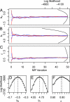
Fig. 3.
Diagnostic plots. (A–C) Convergence plots for four MIFs, shown for three parameters. The dotted line shows θ*. The parabolic lines give the sliced likelihood through θ̂, with the axis scale at the top right. (D–F) Corresponding close-ups of the sliced likelihood. The dashed vertical line is at θ̂.
Fig. 4.
Profile likelihood for the environmental reservoir parameter. The larger of two MIF replications was plotted at each value of ω (circles), maximizing over the other parameters. Local quadratic regression (33, 35) with a bandwidth parameter (span) of 0.5 was used to estimate the profile likelihood (solid line). The dotted lines construct an approximate 99% confidence interval (ref. and Supporting Text) of (75 × 10−6, 210 × 10−6).
Fig. 5.
Superimposed annual cycles of cholera mortality in Dhaka, 1891–1940.
Similar articles
- Estimating parameters and hidden variables in non-linear state-space models based on ODEs for biological networks inference.
Quach M, Brunel N, d'Alché-Buc F. Quach M, et al. Bioinformatics. 2007 Dec 1;23(23):3209-16. doi: 10.1093/bioinformatics/btm510. Bioinformatics. 2007. PMID: 18042557 - Maximum likelihood estimation in dynamical models of HIV.
Guedj J, Thiébaut R, Commenges D. Guedj J, et al. Biometrics. 2007 Dec;63(4):1198-206. doi: 10.1111/j.1541-0420.2007.00812.x. Epub 2007 May 8. Biometrics. 2007. PMID: 17489970 - Identifiability and observability analysis for experimental design in nonlinear dynamical models.
Raue A, Becker V, Klingmüller U, Timmer J. Raue A, et al. Chaos. 2010 Dec;20(4):045105. doi: 10.1063/1.3528102. Chaos. 2010. PMID: 21198117 - Noisy clockwork: time series analysis of population fluctuations in animals.
Bjørnstad ON, Grenfell BT. Bjørnstad ON, et al. Science. 2001 Jul 27;293(5530):638-43. doi: 10.1126/science.1062226. Science. 2001. PMID: 11474099 Review. - Parametric Bayesian filters for nonlinear stochastic dynamical systems: a survey.
Stano P, Lendek Z, Braaksma J, Babuska R, de Keizer C, den Dekker AJ. Stano P, et al. IEEE Trans Cybern. 2013 Dec;43(6):1607-24. doi: 10.1109/TSMCC.2012.2230254. IEEE Trans Cybern. 2013. PMID: 23757593 Review.
Cited by
- PREDICTIVE MODELING OF CHOLERA OUTBREAKS IN BANGLADESH.
Koepke AA, Longini IM Jr, Halloran ME, Wakefield J, Minin VN. Koepke AA, et al. Ann Appl Stat. 2016 Jun;10(2):575-595. doi: 10.1214/16-AOAS908. Epub 2016 Jul 22. Ann Appl Stat. 2016. PMID: 27746850 Free PMC article. - Bayesian history matching of complex infectious disease models using emulation: a tutorial and a case study on HIV in Uganda.
Andrianakis I, Vernon IR, McCreesh N, McKinley TJ, Oakley JE, Nsubuga RN, Goldstein M, White RG. Andrianakis I, et al. PLoS Comput Biol. 2015 Jan 8;11(1):e1003968. doi: 10.1371/journal.pcbi.1003968. eCollection 2015 Jan. PLoS Comput Biol. 2015. PMID: 25569850 Free PMC article. - Comparing and linking machine learning and semi-mechanistic models for the predictability of endemic measles dynamics.
Lau MSY, Becker A, Madden W, Waller LA, Metcalf CJE, Grenfell BT. Lau MSY, et al. PLoS Comput Biol. 2022 Sep 8;18(9):e1010251. doi: 10.1371/journal.pcbi.1010251. eCollection 2022 Sep. PLoS Comput Biol. 2022. PMID: 36074763 Free PMC article. - Dynamic Variation in Sexual Contact Rates in a Cohort of HIV-Negative Gay Men.
Romero-Severson EO, Volz E, Koopman JS, Leitner T, Ionides EL. Romero-Severson EO, et al. Am J Epidemiol. 2015 Aug 1;182(3):255-62. doi: 10.1093/aje/kwv044. Epub 2015 May 20. Am J Epidemiol. 2015. PMID: 25995288 Free PMC article. - Spatial clustering in the spatio-temporal dynamics of endemic cholera.
Ruiz-Moreno D, Pascual M, Emch M, Yunus M. Ruiz-Moreno D, et al. BMC Infect Dis. 2010 Mar 6;10:51. doi: 10.1186/1471-2334-10-51. BMC Infect Dis. 2010. PMID: 20205935 Free PMC article.
References
- Anderson BD, Moore JB. Optimal Filtering. Engelwood Cliffs, NJ: Prentice-Hall; 1979.
- Shephard N, Pitt MK. Biometrika. 1997;84:653–667.
- Ionides EL, Fang KS, Isseroff RR, Oster GF. J Math Biol. 2004;48:23–37. - PubMed
- Houtekamer PL, Mitchell HL. Mon Weather Rev. 2001;129:123–137.
- Thomas L, Buckland ST, Newman KB, Harwood J. Aust NZ J Stat. 2005;47:19–34.
Publication types
MeSH terms
LinkOut - more resources
Full Text Sources
Other Literature Sources
Medical


