Quantitative and qualitative beta diversity measures lead to different insights into factors that structure microbial communities - PubMed (original) (raw)
Quantitative and qualitative beta diversity measures lead to different insights into factors that structure microbial communities
Catherine A Lozupone et al. Appl Environ Microbiol. 2007 Mar.
Abstract
The assessment of microbial diversity and distribution is a major concern in environmental microbiology. There are two general approaches for measuring community diversity: quantitative measures, which use the abundance of each taxon, and qualitative measures, which use only the presence/absence of data. Quantitative measures are ideally suited to revealing community differences that are due to changes in relative taxon abundance (e.g., when a particular set of taxa flourish because a limiting nutrient source becomes abundant). Qualitative measures are most informative when communities differ primarily by what can live in them (e.g., at high temperatures), in part because abundance information can obscure significant patterns of variation in which taxa are present. We illustrate these principles using two 16S rRNA-based surveys of microbial populations and two phylogenetic measures of community beta diversity: unweighted UniFrac, a qualitative measure, and weighted UniFrac, a new quantitative measure, which we have added to the UniFrac website (http://bmf.colorado.edu/unifrac). These studies considered the relative influences of mineral chemistry, temperature, and geography on microbial community composition in acidic thermal springs in Yellowstone National Park and the influences of obesity and kinship on microbial community composition in the mouse gut. We show that applying qualitative and quantitative measures to the same data set can lead to dramatically different conclusions about the main factors that structure microbial diversity and can provide insight into the nature of community differences. We also demonstrate that both weighted and unweighted UniFrac measurements are robust to the methods used to build the underlying phylogeny.
Figures
FIG. 1.
Calculation of the unweighted and the weighted UniFrac measures. Squares and circles represent sequences from two different environments. (a) In unweighted UniFrac, the distance between the circle and square communities is calculated as the fraction of the branch length that has descendants from either the square or the circle environment (black) but not both (gray). (b) In weighted UniFrac, branch lengths are weighted by the relative abundance of sequences in the square and circle communities; square sequences are weighted twice as much as circle sequences because there are twice as many total circle sequences in the data set. The width of branches is proportional to the degree to which each branch is weighted in the calculations, and gray branches have no weight. Branches 1 and 2 have heavy weights since the descendants are biased toward the square and circles, respectively. Branch 3 contributes no value since it has an equal contribution from circle and square sequences after normalization.
FIG. 2.
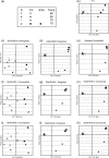
PCoA analysis of hot spring sediment samples with FST and unweighted, weighted, and normalized weighted UniFrac using a variety of trees. Shown is a plot of the first two principal coordinate axes (factors) for PCoA using each tree-building method and a UniFrac algorithm. Rows show the effects of different tree-building methods; columns show the effects of applying unweighted UniFrac (first column), weighted UniFrac (second column), and weighted UniFrac with the branch length normalization (third column). (a) The legend describes which symbol applies to which sample. Fe-containing springs have solid symbols; springs that contain only S have hollow symbols. Temperature (°C) is denoted by the shape of the symbol. (b) PCoA clustering using FST values as distances. (c through e) Neighbor-joining tree from NEIGHBOR. (f through h) and (i through k) Two representative parsimony trees from DNAPARS. (l through n) ARB parsimony insertion tree. (o through q) RAxML maximum likelihood tree. (r through t) RAxML parsimony guide tree, no branch lengths. (u through w) MrBayes consensus tree.
FIG. 3.
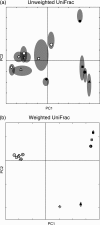
Jackknifing of PCoA analysis of hot spring sediment samples with unweighted and weighted UniFrac. Shown is a plot of the first two principal coordinate axes (factors) for PCoA with the neighbor-joining tree. Point locations are the average location in the 100 jackknife replicates. Only 50 randomly selected sequences from each sample were used in each replicate (the range of sequences per sample was 65 to 96). Gray ellipses represent the IQR for the 100 jackknife replicates. The 95% confidence intervals for the point locations were also calculated and were considerably smaller than the IQRs (data not shown). The symbols are the same as those shown in Fig. 2.
FIG. 4.
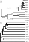
Hierarchical clustering of hot spring sediment samples with weighted and unweighted UniFrac. The percentage support for nodes supported at least 70% of the time with sequence jackknifing is indicated. The name of each sample indicates the spring (e.g., A1, A2, and A3 are different springs from the Amphitheatre Springs area, and RM is from the Roaring Mountain area), whether the sample is sulfur rich (S), iron rich (Fe), or both (FeS), and the temperature. The names and branches are colored black for S samples and gray for Fe and FeS samples. (a) Weighted UniFrac with the neighbor-joining tree and (b) unweighted UniFrac with the neighbor-joining tree.
FIG. 5.
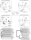
Analysis of mouse cecal microbial communities with weighted and unweighted UniFrac. Genotypes are ob/ob for homozygotes for the mutant leptin allele that confers obesity, ob/+ for heterozygotes, and +/+ for wild types. All mothers are ob/+. (a) Plot of the first two principal coordinate axes for PCoA with unweighted UniFrac. Symbols represent individual animals. The rectangles highlight the family of mother 2 and the families of mothers 1 and 3, who are sisters. (b) The same plot for weighted Unifrac. The rectangle highlights the majority of the ob/ob mice. The arrows point to outliers: an ob/ob mouse outside of the ob/ob cluster (black triangle) and an ob/+ mouse inside the ob/ob cluster (white square). (c) Same plot for sequence jackknifing of unweighted UniFrac with a maximum of 200 sequences from each mouse for 100 replicates. The symbols are the average values for the 100 replicates, and the gray ellipses represent the IQR of the point locations. (d) Sequence jackknifing with weighted UniFrac with a maximum of 200 sequences from each mouse for 100 replicates. (e) Hierarchical cluster diagram for unweighted UniFrac. The percentage support for nodes supported at least 70% of the time with sequence jackknifing is indicated. The main clustering is by mother. (f) Hierarchical cluster diagram for weighted UniFrac. The clustering by mother is much less clear, and there is more clustering by ob/ob genotype (and hence by obesity phenotype).
Similar articles
- Effects of abiotic factors on the phylogenetic diversity of bacterial communities in acidic thermal springs.
Mathur J, Bizzoco RW, Ellis DG, Lipson DA, Poole AW, Levine R, Kelley ST. Mathur J, et al. Appl Environ Microbiol. 2007 Apr;73(8):2612-23. doi: 10.1128/AEM.02567-06. Epub 2007 Jan 12. Appl Environ Microbiol. 2007. PMID: 17220248 Free PMC article. - UniFrac--an online tool for comparing microbial community diversity in a phylogenetic context.
Lozupone C, Hamady M, Knight R. Lozupone C, et al. BMC Bioinformatics. 2006 Aug 7;7:371. doi: 10.1186/1471-2105-7-371. BMC Bioinformatics. 2006. PMID: 16893466 Free PMC article. - Bacteria and Archaea diversity within the hot springs of Lake Magadi and Little Magadi in Kenya.
Kambura AK, Mwirichia RK, Kasili RW, Karanja EN, Makonde HM, Boga HI. Kambura AK, et al. BMC Microbiol. 2016 Jul 7;16(1):136. doi: 10.1186/s12866-016-0748-x. BMC Microbiol. 2016. PMID: 27388368 Free PMC article. - Phylogenetic approaches for describing and comparing the diversity of microbial communities.
Martin AP. Martin AP. Appl Environ Microbiol. 2002 Aug;68(8):3673-82. doi: 10.1128/AEM.68.8.3673-3682.2002. Appl Environ Microbiol. 2002. PMID: 12147459 Free PMC article. Review. No abstract available. - Species divergence and the measurement of microbial diversity.
Lozupone CA, Knight R. Lozupone CA, et al. FEMS Microbiol Rev. 2008 Jul;32(4):557-78. doi: 10.1111/j.1574-6976.2008.00111.x. Epub 2008 Apr 22. FEMS Microbiol Rev. 2008. PMID: 18435746 Free PMC article. Review.
Cited by
- Navy Bean Supplementation in Established High-Fat Diet-Induced Obesity Attenuates the Severity of the Obese Inflammatory Phenotype.
Monk JM, Wu W, Lepp D, Pauls KP, Robinson LE, Power KA. Monk JM, et al. Nutrients. 2021 Feb 26;13(3):757. doi: 10.3390/nu13030757. Nutrients. 2021. PMID: 33652785 Free PMC article. - Effect of 15 days -6° head-down bed rest on microbial communities of supragingival plaque in young men.
Zhu D, Qiao P, Zhou Q, Sun H, Xin B, Wu B, Tang C. Zhu D, et al. Front Microbiol. 2024 Jan 24;15:1331023. doi: 10.3389/fmicb.2024.1331023. eCollection 2024. Front Microbiol. 2024. PMID: 38328428 Free PMC article. - Maternal IgG and IgA Antibodies Dampen Mucosal T Helper Cell Responses in Early Life.
Koch MA, Reiner GL, Lugo KA, Kreuk LS, Stanbery AG, Ansaldo E, Seher TD, Ludington WB, Barton GM. Koch MA, et al. Cell. 2016 May 5;165(4):827-41. doi: 10.1016/j.cell.2016.04.055. Cell. 2016. PMID: 27153495 Free PMC article. - Abiotic factors shape microbial diversity in Sonoran Desert soils.
Andrew DR, Fitak RR, Munguia-Vega A, Racolta A, Martinson VG, Dontsova K. Andrew DR, et al. Appl Environ Microbiol. 2012 Nov;78(21):7527-37. doi: 10.1128/AEM.01459-12. Epub 2012 Aug 10. Appl Environ Microbiol. 2012. PMID: 22885757 Free PMC article. - Surveying the microbiome of ants: comparing 454 pyrosequencing with traditional methods to uncover bacterial diversity.
Kautz S, Rubin BE, Russell JA, Moreau CS. Kautz S, et al. Appl Environ Microbiol. 2013 Jan;79(2):525-34. doi: 10.1128/AEM.03107-12. Epub 2012 Nov 2. Appl Environ Microbiol. 2013. PMID: 23124239 Free PMC article.
References
- Badano, E. I., and L. A. Cavieres. 2006. Impacts of ecosystem engineers on community attributes: effects of cushion plants at different elevations of the Chilean Andes. Divers. Distrib. 12:388-396.
- Bluis, J., and D. Shin. 2003. Nodal distance algorithm: calculating a phylogenetic tree comparison metric, p. 87-94. In Proceedings of the Third IEEE Symposium on BioInformatics and BioEngineering. IEEE, Los Alamitos, CA.
- De Benedictis, P. A. 1973. On the correlations between certain diversity indices. Am. Nat. 107:295-302.
- Felsenstein, J. 2004. Inferring phylogenies. Sinauer Associates, Inc., Sunderland, MA.
Publication types
MeSH terms
Substances
Grants and funding
- T32 GM008759/GM/NIGMS NIH HHS/United States
- T32 GM065103/GM/NIGMS NIH HHS/United States
- T32 GM142607/GM/NIGMS NIH HHS/United States
- T32 GM08759/GM/NIGMS NIH HHS/United States
LinkOut - more resources
Full Text Sources


