Parameter estimation for robust HMM analysis of ChIP-chip data - PubMed (original) (raw)
Parameter estimation for robust HMM analysis of ChIP-chip data
Peter Humburg et al. BMC Bioinformatics. 2008.
Abstract
Background: Tiling arrays are an important tool for the study of transcriptional activity, protein-DNA interactions and chromatin structure on a genome-wide scale at high resolution. Although hidden Markov models have been used successfully to analyse tiling array data, parameter estimation for these models is typically ad hoc. Especially in the context of ChIP-chip experiments, no standard procedures exist to obtain parameter estimates from the data. Common methods for the calculation of maximum likelihood estimates such as the Baum-Welch algorithm or Viterbi training are rarely applied in the context of tiling array analysis.
Results: Here we develop a hidden Markov model for the analysis of chromatin structure ChIP-chip tiling array data, using t emission distributions to increase robustness towards outliers. Maximum likelihood estimates are used for all model parameters. Two different approaches to parameter estimation are investigated and combined into an efficient procedure.
Conclusion: We illustrate an efficient parameter estimation procedure that can be used for HMM based methods in general and leads to a clear increase in performance when compared to the use of ad hoc estimates. The resulting hidden Markov model outperforms established methods like TileMap in the context of histone modification studies.
Figures
Figure 1
Hidden Markov model for the analysis of ChIP-chip tiling array data.
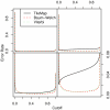
Figure 2
Error rate for different models on datasets I and II. Error rate resulting from the different models on dataset I (left) and II (right). When the total number of incorrect probe calls is considered, both parameter estimation procedures outperform TileMap on dataset I for cut-offs larger than 0.2. Both Baum-Welch and Viterbi training provide models with an optimal cut-off close to 0.5, while TileMap significantly underestimates the posterior probability resulting in an optimal cut-off of 0.19. The models with optimised parameters show similar performance on both datasets. On dataset II TileMap's performance is reduced in comparison to the results on dataset I. The main differences between the models considered here occur at error rates of 0–0.08. The relevant area of the figures in the top row is magnified in the plots below.
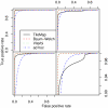
Figure 3
ROC curves for different models on datasets I and II. TileMap and the models with Baum-Welch and Viterbi training parameter estimates show similar performance on dataset I (left) with a small advantage for the models with optimised parameters. Comparison with a model using ad hoc parameter estimates highlights the performance increase achieved by optimising model parameters. On dataset II (right) TileMap performs similarly to the model with ad hoc parameter estimates. Figures on the bottom provide a close-up view of the plots above.
Figure 4
Model performance for different choices of ν. The Baum-Welch model (red) performs better for relatively small values of ν while Viterbi training (blue) favours larger ν. For the optimal choice of ν the Baum-Welch parameter estimates lead to an optimal cut-off close to 0.5.
Figure 5
AUC for different choices of ν and increasing numberof iterations. Change in AUC for different choices of ν (left). The Baum-Welch model performs better for relatively small values of ν while Viterbi training favours larger ν. Improvements in AUC with increasing number of iterations (right). The performance of the Viterbi trained model improves substantially during the first five iterations. Further iterations only produce small changes in the AUC. The Baum-Welch method requires more iterations to obtain the same AUC as as the Viterbi model. After 20 iterations the Baum-Welch model starts to outperform the Viterbi model.
Figure 6
Error rate at optimal and 0.5 cutoff for increasing number of iterations. Parameter estimates obtained by the Baum-Welch algorithm (filled symbols) and Viterbi training (open symbols) improve model performance with increasing nuber of iterations. Viterbi training quickly approaches its optimal solution and initially outperforms Baum-Welch. The final model produced by the Baum-Welch algorithm provides a lower error rate than Viterbi training.
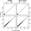
Figure 7
Length distribution of enriched regions from dataset I. Quantile-quantile plots comparing length distributions of enriched regions found with TileMap (left) and with the model based on maximum likelihood estimates (right) to the true length distribution of enriched regions in dataset I. Figures on the bottom provide a close-up view of the plots above. Each dot represents a percentile of the length distributions.
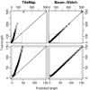
Figure 8
Length distribution of enriched regions from dataset II. Quantile-quantile plots comparing length distributions of enriched regions found with TileMap (left) and with the model based on maximum likelihood estimates (right) to the true length distribution of enriched regions in dataset II. Figures on the bottom provide a close-up view of the plots above. Each dot represents a percentile of the length distributions.
Figure 9
Analysis of ChIP-chip data. (a) Gene density in areas surrounding genes that contain H3K27me3 enriched regions and genes that do not contain enriched regions. (b) Number of genes found in H3K27me3 regions. While most enriched regions cover a single gene, there is a substantial number of H3K27me3 regions that cover several genes and enriched regions are found to contain up to seven genes. (c) Length distribution of H3K27me3 regions.
Figure 10
Length distribution of enriched regions from real data. Length distribution of enriched regions as determined by TileMap (blue) and Baum-Welch (red). Region length is determined in terms of probes per region. Both distributions were truncated at 10 for the simulation, ensuring that all regions in the simulated data contain at least ten probes.
Similar articles
- A supervised hidden markov model framework for efficiently segmenting tiling array data in transcriptional and chIP-chip experiments: systematically incorporating validated biological knowledge.
Du J, Rozowsky JS, Korbel JO, Zhang ZD, Royce TE, Schultz MH, Snyder M, Gerstein M. Du J, et al. Bioinformatics. 2006 Dec 15;22(24):3016-24. doi: 10.1093/bioinformatics/btl515. Epub 2006 Oct 12. Bioinformatics. 2006. PMID: 17038339 - Implementing EM and Viterbi algorithms for Hidden Markov Model in linear memory.
Churbanov A, Winters-Hilt S. Churbanov A, et al. BMC Bioinformatics. 2008 Apr 30;9:224. doi: 10.1186/1471-2105-9-224. BMC Bioinformatics. 2008. PMID: 18447951 Free PMC article. - A hidden Ising model for ChIP-chip data analysis.
Mo Q, Liang F. Mo Q, et al. Bioinformatics. 2010 Mar 15;26(6):777-83. doi: 10.1093/bioinformatics/btq032. Epub 2010 Jan 28. Bioinformatics. 2010. PMID: 20110277 - Continuous-index hidden Markov modelling of array CGH copy number data.
Stjernqvist S, Rydén T, Sköld M, Staaf J. Stjernqvist S, et al. Bioinformatics. 2007 Apr 15;23(8):1006-14. doi: 10.1093/bioinformatics/btm059. Epub 2007 Feb 19. Bioinformatics. 2007. PMID: 17309894 - Modeling and analysis of ChIP-chip experiments.
Gottardo R. Gottardo R. Methods Mol Biol. 2009;567:133-43. doi: 10.1007/978-1-60327-414-2_9. Methods Mol Biol. 2009. PMID: 19588090 Review.
Cited by
- Global analysis of the relationship between JIL-1 kinase and transcription.
Regnard C, Straub T, Mitterweger A, Dahlsveen IK, Fabian V, Becker PB. Regnard C, et al. PLoS Genet. 2011 Mar;7(3):e1001327. doi: 10.1371/journal.pgen.1001327. Epub 2011 Mar 10. PLoS Genet. 2011. PMID: 21423663 Free PMC article. - Detection of epigenetic changes using ANOVA with spatially varying coefficients.
Guanghua X, Xinlei W, Quincey L, Nestler EJ, Xie Y. Guanghua X, et al. Stat Appl Genet Mol Biol. 2013 Mar 13;12(2):189-205. doi: 10.1515/sagmb-2012-0057. Stat Appl Genet Mol Biol. 2013. PMID: 23502341 Free PMC article. - Hierarchical hidden Markov model with application to joint analysis of ChIP-chip and ChIP-seq data.
Choi H, Nesvizhskii AI, Ghosh D, Qin ZS. Choi H, et al. Bioinformatics. 2009 Jul 15;25(14):1715-21. doi: 10.1093/bioinformatics/btp312. Epub 2009 May 14. Bioinformatics. 2009. PMID: 19447789 Free PMC article. - MultiChIPmixHMM: an R package for ChIP-chip data analysis modeling spatial dependencies and multiple replicates.
Bérard C, Seifert M, Mary-Huard T, Martin-Magniette ML. Bérard C, et al. BMC Bioinformatics. 2013 Sep 9;14:271. doi: 10.1186/1471-2105-14-271. BMC Bioinformatics. 2013. PMID: 24015679 Free PMC article. - Open chromatin structures regulate the efficiencies of pre-RC formation and replication initiation in Epstein-Barr virus.
Papior P, Arteaga-Salas JM, Günther T, Grundhoff A, Schepers A. Papior P, et al. J Cell Biol. 2012 Aug 20;198(4):509-28. doi: 10.1083/jcb.201109105. Epub 2012 Aug 13. J Cell Biol. 2012. PMID: 22891264 Free PMC article.
References
- Cawley S, Bekiranov S, Ng HH, Kapranov P, Sekinger EA, Kampa D, Piccolboni A, Sementchenko V, Cheng J, Williams AJ, Wheeler R, Wong B, Drenkow J, Yamanaka M, Patel S, Brubaker S, Tammana H, Helt G, Struhl K, Gingeras TR. Unbiased Mapping of Transcription Factor Binding Sites along Human Chromosomes 21 and 22 Points to Widespread Regulation of Noncoding RNAs. Cell. 2004;116:499–509. doi: 10.1016/S0092-8674(04)00127-8. - DOI - PubMed
- Bernstein BE, Kamal M, Lindblad-Toh K, Bekiranov S, Bailey DK, Huebert DJ, McMahon S, Karlsson EK, III EJK, Gingeras TR, Schreiber SL, Lander ES. Genomic Maps and Comparative Analysis of Histone Modifications in Human and Mouse. Cell. 2005;120:169–181. doi: 10.1016/j.cell.2005.01.001. - DOI - PubMed
Publication types
MeSH terms
LinkOut - more resources
Full Text Sources
Molecular Biology Databases


