An approach for extensibly profiling the molecular states of cellular subpopulations - PubMed (original) (raw)
An approach for extensibly profiling the molecular states of cellular subpopulations
Lit-Hsin Loo et al. Nat Methods. 2009 Oct.
Abstract
Microscopy often reveals the existence of phenotypically distinct cellular subpopulations. However, additional characterization of observed subpopulations can be limited by the number of biomolecular markers that can be simultaneously monitored. Here we present a computational approach for extensibly profiling cellular subpopulations by freeing one or more imaging channels to monitor additional probes. In our approach, we trained classifiers to re-identify subpopulations accurately based on an enhanced collection of phenotypic features extracted from only a subset of the original markers. Then we constructed subpopulation profiles step-wise from replicate experiments, in which cells were labeled with different but overlapping marker sets. We applied our approach to identify molecular differences among subpopulations and to identify functional groupings of markers, in populations of differentiating mouse preadipocytes, polarizing human neutrophil-like cells and dividing human cancer cells.
Figures
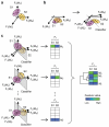
Figure 1. Building extensible Virtual Phenotypic Profiles of cellular subpopulations
Schematic showing the three major steps: (a) Step 1, stain and image cells with an initial biomolecular marker set (MA, MB, and MC), and identify subpopulations based on an initial phenotypic feature set (F1, F2, and F3). (b) Step 2, free up an imaging channel by dropping a marker (MC), and adding more high-content features (F4 and F5) to partially compensate for the information lost. Train a classifier based on the new “reference” feature set to separate subpopulations. (c) Step 3, co-stain cells with the reduced marker set (MA and MB) and new markers (MD, ME, … , MZ), and use the trained classifier to separate cells into subpopulations. For each subpopulation, measure the averaged values of a specific chosen feature (Fs) for every marker, and combine the values into a common Virtual Phenotypic Profile. (Fi(Mj) = phenotypic feature i based on marker j; S1, S2 = subpopulations 1 and 2; pink and yellow squares = cells from S1 and S2; ellipsoids = boundaries of subpopulations; dashed lines or hyperplanes = trained classifiers)
Figure 2. High-content features partially compensated the decrease in classification performance due to dropping a marker
(a) Immunofluorescence images of 3T3-L1 cells near the centroids of the four identified 3T3-L1 subpopulations (S1 to S4) during adipogenesis. White curves = automated segmentation boundaries; scale bar = 20 μm. (b) 2D scatter plot showing the Day 9 distribution of the subpopulations identified based on LD and AdipoQ levels. The percentages of cells are shown in parentheses. Data shown was 25% sub-sampled for visualization (triangles = subpopulation centroids). (c) Average minimum class accuracy (MCA) of subpopulation classification after systematic dropping of each initial marker. The accuracies for the best classifier type for each feature set (Supplementary Fig. 1a) are shown. (d) Average MCA of subpopulation classification after dropping the LD marker, and adding high-content features from the AdipoQ marker. Shown are the accuracies for the best overall classifier type, SVM-RBF classifier (Supplementary Fig. 1b). All features implicitly contain information from the DNA marker, which was used for segmentation. (INT/ALL = all initial features; INT/AdipoQ = initial adiponectin feature, INT/LD = initial LD feature; HC/ALL = all additional high-content features; HC/SFFS = high-content feature subset selected by sequential floating forward search; error bars = standard errors of cross-validation; ** = P<0.010; *** = P<0.001; one-sided paired _t_-test; n = 3)
Figure 3. Virtual Phenotypic Profiles had low noise levels and were significantly different from population averages
(a) Distributions of the nuclear or cellular levels of five new markers in subpopulations identified based on all initial features (INT/ALL), initial adiponectin feature alone (INT/AdipoQ), or high-content adiponectin features (HC/SFFS). (PPARγ = peroxisome proliferator-activated receptor gamma; C/EBPα = CCAAT/enhancer binding protein alpha; PLINA = perilipin A; HSL = hormone sensitive lipase; pHSL = HSL phosphorylated at S565; error bars = medians ± upper and lower quartiles). (b) Absolute noise levels of the median cellular levels for the dropped marker (LD, left subpanel) and a new marker (PLINA, right subpanel) on subpopulations identified from either INT/AdipoQ or HC/SFFS (error bars = means ± standard errors; ** = P<0.01; *** = P<0.001; one-sided paired t-test; n = 3.) (c) Number of initial markers (left subpanel) or new markers (right subpanel) with HC/SFFS noise level significantly lower than INT/AdipoQ noise level (one-sided paired t-test; n = 3). (d) Multi-dimensional scaling plot showing the relative distances of the Virtual Phenotypic Profiles of the four identified subpopulations identified from HC/SFFS to the profiles of the whole cellular population, or randomly-selected subpopulations. P-value shown was the probability that a profile may be obtained from randomly selected subpopulations (Supplementary Methods).
Figure 4. High-content features from AdipoQ gave similar clustering and heatmap of Virtual Phenotypic Profiles as the initial features
Dendrograms and heatmaps showing the hierarchical clustering of the normalized Virtual Phenotypic Profiles for the subpopulations identified based on either (a) all the initial features (INT/ALL), (b) initial adiponectin feature alone (INT/AdipoQ), or (c) high-content adiponectin features (HC/SFFS). The profile of each marker was normalized by dividing the profile with its maximum value. The known functions of the tested biomolecules are indicated. The distance metric used was Euclidean distance, and the clustering algorithm used was average linkage.
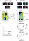
Figure 5. Virtual Phenotypic Profiling of polarizing and of dividing cells
(a) Immunofluorescence images showing polarizing HL-60 cells near the centroids of the three identified subpopulations, S1, S2, and S3 (white curves = automated segmentation boundaries; scale bar = 20 μm). (b) Dendrogram and heatmap of normalized Virtual Phenotypic Profiles showing the hierarchical clustering of the biomolecules based on polarization indices and F-actin co-localization (Supplementary Methods). The known functions of the biomolecules are indicated (pPTEN = phosphorylated phosphatase and tensin homolog; pAKT = phosphorylated AKT; Hem1 = hematopoietic protein 1). (c) 2D scatter plot of the original (un-normalized) Virtual Phenotypic Profile for S3 cells showed that molecules from related pathways had similar values of polarization index and F-actin co-localization. (d) Immunofluorescence images showing dividing H460 cells near the centroids of the four identified subpopulations, S1, S2, S3, and S4 (corresponding to G1, S, G2 and M-phase cells respectively; white curves = automated segmentation boundaries; scale bar = 20 μm). (e) Dendrogram and heatmap of normalized Virtual Phenotypic Profiles showing the hierarchical clustering of biomolecules based on their total cellular levels in different subpopulations (pRb = phosphorylated retinoblastoma protein). (f) 2D scatter plots of the Virtual Phenotypic Profiles showing subcellular localization relative to DNA and expression levels of the tested biomolecules in different phases of the cell cycle.
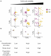
Figure 6. Effectiveness of subpopulation profiling depends on the degree of cell-to-cell variability
(a) Simulated co-staining levels of a set of biomolecular markers on individual cells at different degrees of cell-to-cell variability (as measured by the average cell-to-cell dissimilarity). Fref, a reference feature used to divide the cells into two subpopulations. Fs, a specific feature of marker A or B. (dashed line = decision boundary of the classifier used.) (b) Medians and interquartile ranges of the single-cell distributions of Fs in each of the two subpopulations. These features formed the basis for the Virtual Phenotypic Profiles (error bars = interquartile ranges.) (c) The effectiveness of subpopulation profiling evaluated using three criteria.
Similar articles
- A dynamic programming approach for the alignment of signal peaks in multiple gas chromatography-mass spectrometry experiments.
Robinson MD, De Souza DP, Keen WW, Saunders EC, McConville MJ, Speed TP, Likić VA. Robinson MD, et al. BMC Bioinformatics. 2007 Oct 29;8:419. doi: 10.1186/1471-2105-8-419. BMC Bioinformatics. 2007. PMID: 17963529 Free PMC article. - Multiclass cancer classification and biomarker discovery using GA-based algorithms.
Liu JJ, Cutler G, Li W, Pan Z, Peng S, Hoey T, Chen L, Ling XB. Liu JJ, et al. Bioinformatics. 2005 Jun 1;21(11):2691-7. doi: 10.1093/bioinformatics/bti419. Epub 2005 Apr 6. Bioinformatics. 2005. PMID: 15814557 - Clustering-based spot segmentation of cDNA microarray images.
Uslan V, Bucak IÖ. Uslan V, et al. Annu Int Conf IEEE Eng Med Biol Soc. 2010;2010:1828-31. doi: 10.1109/IEMBS.2010.5626430. Annu Int Conf IEEE Eng Med Biol Soc. 2010. PMID: 21096143 - How does gene expression clustering work?
D'haeseleer P. D'haeseleer P. Nat Biotechnol. 2005 Dec;23(12):1499-501. doi: 10.1038/nbt1205-1499. Nat Biotechnol. 2005. PMID: 16333293 Review. - Unsupervised pattern recognition: an introduction to the whys and wherefores of clustering microarray data.
Boutros PC, Okey AB. Boutros PC, et al. Brief Bioinform. 2005 Dec;6(4):331-43. doi: 10.1093/bib/6.4.331. Brief Bioinform. 2005. PMID: 16420732 Review.
Cited by
- Capturing cell heterogeneity in representations of cell populations for image-based profiling using contrastive learning.
van Dijk R, Arevalo J, Babadi M, Carpenter AE, Singh S. van Dijk R, et al. bioRxiv [Preprint]. 2024 Jul 31:2023.11.14.567038. doi: 10.1101/2023.11.14.567038. bioRxiv. 2024. PMID: 39131344 Free PMC article. Updated. Preprint. - Systematic data analysis pipeline for quantitative morphological cell phenotyping.
Ghanegolmohammadi F, Eslami M, Ohya Y. Ghanegolmohammadi F, et al. Comput Struct Biotechnol J. 2024 Jul 14;23:2949-2962. doi: 10.1016/j.csbj.2024.07.012. eCollection 2024 Dec. Comput Struct Biotechnol J. 2024. PMID: 39104709 Free PMC article. Review. - A statistical framework for high-content phenotypic profiling using cellular feature distributions.
Pearson YE, Kremb S, Butterfoss GL, Xie X, Fahs H, Gunsalus KC. Pearson YE, et al. Commun Biol. 2022 Dec 22;5(1):1409. doi: 10.1038/s42003-022-04343-3. Commun Biol. 2022. PMID: 36550289 Free PMC article. - Image-based cell profiling enhancement via data cleaning methods.
Rezvani A, Bigverdi M, Rohban MH. Rezvani A, et al. PLoS One. 2022 May 4;17(5):e0267280. doi: 10.1371/journal.pone.0267280. eCollection 2022. PLoS One. 2022. PMID: 35507559 Free PMC article. - Single-cell lipidomics with high structural specificity by mass spectrometry.
Li Z, Cheng S, Lin Q, Cao W, Yang J, Zhang M, Shen A, Zhang W, Xia Y, Ma X, Ouyang Z. Li Z, et al. Nat Commun. 2021 May 17;12(1):2869. doi: 10.1038/s41467-021-23161-5. Nat Commun. 2021. PMID: 34001877 Free PMC article.
References
- Gallin JI. Human neutrophil heterogeneity exists, but is it meaningful? Blood. 1984;63:977–983. - PubMed
- Rubin H. The significance of biological heterogeneity. Cancer Metastasis Rev. 1990;9:1–20. - PubMed
Publication types
MeSH terms
Substances
Grants and funding
- R01 GM081549/GM/NIGMS NIH HHS/United States
- R01 GM081549-02/GM/NIGMS NIH HHS/United States
- R01 GM085442-02/GM/NIGMS NIH HHS/United States
- R01 GM085442/GM/NIGMS NIH HHS/United States
- R01 GM085442-01/GM/NIGMS NIH HHS/United States
- R01 GM081549-03/GM/NIGMS NIH HHS/United States
LinkOut - more resources
Full Text Sources


