Classification of structural heterogeneity by maximum-likelihood methods - PubMed (original) (raw)
Classification of structural heterogeneity by maximum-likelihood methods
Sjors H W Scheres. Methods Enzymol. 2010.
Abstract
With the advent of computationally feasible approaches to maximum-likelihood (ML) image processing for cryo-electron microscopy, these methods have proven particularly useful in the classification of structurally heterogeneous single-particle data. A growing number of experimental studies have applied these algorithms to study macromolecular complexes with a wide range of structural variability, including nonstoichiometric complex formation, large conformational changes, and combinations of both. This chapter aims to share the practical experience that has been gained from the application of these novel approaches. Current insights on how to prepare the data and how to perform two- or three-dimensional classifications are discussed together with the aspects related to high-performance computing. Thereby, this chapter will hopefully be of practical use for those microscopists wishing to apply ML methods in their own investigations.
Copyright © 2010 Elsevier Inc. All rights reserved.
Figures
Figure 1
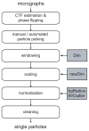
Schematic view of a typical image preprocessing workflow. Important parameters that are discussed in the main text are highlighted in grey. These are the dimension of the boxed particles (Dim), the dimension of the downscaled particles (newDim), the radius of the circle that determines the particle noise area (bgRadius) and the threshold in standard deviations of the image that is used to discard outlier pixel values (thrOutlier).
Figure 2
An illustration of image normalization. All pixels outside the white circle in the upper right image are assumed to contain only noise. These pixels are used to fit a least-squares background plane and to calculate the standard deviation of the noise. The upper row shows original images as they were extracted from the micrographs. The two images on the left show ramping backgrounds, the two images on the right show pixels with extremely low (i.e. black) intensity values. The lower row shows the same four images after normalization.
Figure 3
The results of automated image sorting based on average Z-scores. The top row shows images with relatively low Z-scores, the middle row images with average Z-scores and the bottom row shows images with relatively high Z-scores. The number of bad particles typically increases with higher Z-scores, which may facilitate the interactive removal of outliers by the user.
Figure 4
Schematic view of the use of the ML2D (A) and kerdenSOM (B) algorithms. Important parameters that are discussed in the main text are highlighted in grey. These are the number of classes to be used in ML2D classification (K) and the size of the map (mapSize) and its regularization parameters (regParam) for the kerdenSOM algorithm.
Figure 5
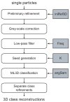
Schematic view of the ML3D classification workflow. Important parameters that are discussed in the main text are highlighted in grey. These are the initial 3D model (iniRef3D), the frequency of the low-pass filter (Freq), and the number of classes (K) and the angular sampling (angSam) to be used in the ML3D refinement.
Figure 6
An example of model bias affecting ML3D classification. Using a suboptimal initial reference (A), ML3D classification yielded suboptimal results (B). Using an improved initial model (C), ML3D classification separated uncomplexed CCT from CCT:Hsc70NBD complexes. See (Cuellar et al., 2008) for more details.
Figure 7
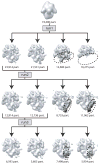
An example of hierarchical classification by ML3D. In three consecutive runs (run 1–3) ML3D classification is used to separate a dataset of 74,400 ribosome particles into multiple classes. Run1 separates intact ribosomes from disintegrated, 50S particles; run2 separates particles with strong density for tmRNA and run3 classifies the remaining intact ribosomes into particles without apparent tmRNA density and particles with weak tmRNA density in an alternative conformation. See (Cheng et al., 2010) for more details.
Figure 8
An illustration of the use of difference maps in the analysis of distinct structural classes. Side-by-side visualization of maps rendered at the same threshold does not readily reveal the structural differences between them (A). Positive (black) and negative (white) difference maps rendered at five standard deviations better reveal compositional and conformational differences (B).
Similar articles
- Processing of Structurally Heterogeneous Cryo-EM Data in RELION.
Scheres SH. Scheres SH. Methods Enzymol. 2016;579:125-57. doi: 10.1016/bs.mie.2016.04.012. Epub 2016 May 31. Methods Enzymol. 2016. PMID: 27572726 Review. - SubspaceEM: A fast maximum-a-posteriori algorithm for cryo-EM single particle reconstruction.
Dvornek NC, Sigworth FJ, Tagare HD. Dvornek NC, et al. J Struct Biol. 2015 May;190(2):200-14. doi: 10.1016/j.jsb.2015.03.009. Epub 2015 Mar 31. J Struct Biol. 2015. PMID: 25839831 Free PMC article. - Structural Study of Heterogeneous Biological Samples by Cryoelectron Microscopy and Image Processing.
White HE, Ignatiou A, Clare DK, Orlova EV. White HE, et al. Biomed Res Int. 2017;2017:1032432. doi: 10.1155/2017/1032432. Epub 2017 Jan 15. Biomed Res Int. 2017. PMID: 28191458 Free PMC article. Review. - Likelihood-based structural analysis of electron microscopy images.
Cossio P, Hummer G. Cossio P, et al. Curr Opin Struct Biol. 2018 Apr;49:162-168. doi: 10.1016/j.sbi.2018.03.004. Epub 2018 Mar 24. Curr Opin Struct Biol. 2018. PMID: 29579548 Review. - Image Processing in Cryo-Electron Microscopy of Single Particles: The Power of Combining Methods.
Sorzano COS, Jiménez-Moreno A, Maluenda D, Ramírez-Aportela E, Martínez M, Cuervo A, Melero R, Conesa JJ, Sánchez-García R, Strelak D, Filipovic J, Fernández-Giménez E, de Isidro-Gómez F, Herreros D, Conesa P, Del Caño L, Fonseca Y, de la Morena JJ, Macías JR, Losana P, Marabini R, Carazo JM. Sorzano COS, et al. Methods Mol Biol. 2021;2305:257-289. doi: 10.1007/978-1-0716-1406-8_13. Methods Mol Biol. 2021. PMID: 33950394
Cited by
- Evolution of standardization and dissemination of cryo-EM structures and data jointly by the community, PDB, and EMDB.
Chiu W, Schmid MF, Pintilie GD, Lawson CL. Chiu W, et al. J Biol Chem. 2021 Jan-Jun;296:100560. doi: 10.1016/j.jbc.2021.100560. Epub 2021 Mar 18. J Biol Chem. 2021. PMID: 33744287 Free PMC article. Review. - Functional conformations for pyruvate carboxylase during catalysis explored by cryoelectron microscopy.
Lasso G, Yu LP, Gil D, Lázaro M, Tong L, Valle M. Lasso G, et al. Structure. 2014 Jun 10;22(6):911-22. doi: 10.1016/j.str.2014.04.011. Epub 2014 May 29. Structure. 2014. PMID: 24882745 Free PMC article. - Mechanisms of ribosome stalling by SecM at multiple elongation steps.
Zhang J, Pan X, Yan K, Sun S, Gao N, Sui SF. Zhang J, et al. Elife. 2015 Dec 14;4:e09684. doi: 10.7554/eLife.09684. Elife. 2015. PMID: 26670735 Free PMC article. - Analysis of the Conformational Landscape of the N-Domains of the AAA ATPase p97: Disentangling the Continuous Conformational Variability in Partially Symmetrical Complexes.
Valimehr S, Vuillemot R, Kazemi M, Jonic S, Rouiller I. Valimehr S, et al. Int J Mol Sci. 2024 Mar 16;25(6):3371. doi: 10.3390/ijms25063371. Int J Mol Sci. 2024. PMID: 38542345 Free PMC article. - Likelihood-based classification of cryo-EM images using FREALIGN.
Lyumkis D, Brilot AF, Theobald DL, Grigorieff N. Lyumkis D, et al. J Struct Biol. 2013 Sep;183(3):377-388. doi: 10.1016/j.jsb.2013.07.005. Epub 2013 Jul 17. J Struct Biol. 2013. PMID: 23872434 Free PMC article.
References
- Al-Amoudi A, Diez DC, Betts MJ, Frangakis AS. The molecular architecture of cadherins in native epidermal desmosomes. Nature. 2007;450:832–837. - PubMed
- Bilbao-Castro J, Marabini R, Sorzano C, Garcia I, Carazo J, Fernandez J. Exploiting desktop supercomputing for three-dimensional electron microscopy reconstructions using ART with blobs. J Struct Biol. 2009;165:19–26. - PubMed
- Cheng K, Ivanova N, Scheres SH, Pavlov MY, Carazo JM, Hebert H, Ehrenberg M, Lindahl M. tmRNASmpB complex mimics native aminoacyl-tRNAs in the a site of stalled ribosomes. J Struct Biol. 2010;169:342–348. - PubMed
Publication types
MeSH terms
Grants and funding
- MC_UP_A025_1013/MRC_/Medical Research Council/United Kingdom
- R01 HL070472/HL/NHLBI NIH HHS/United States
- R01 HL070472-08/HL/NHLBI NIH HHS/United States
- R01HL070472/HL/NHLBI NIH HHS/United States
LinkOut - more resources
Full Text Sources


