A whole-cell computational model predicts phenotype from genotype - PubMed (original) (raw)
A whole-cell computational model predicts phenotype from genotype
Jonathan R Karr et al. Cell. 2012.
Abstract
Understanding how complex phenotypes arise from individual molecules and their interactions is a primary challenge in biology that computational approaches are poised to tackle. We report a whole-cell computational model of the life cycle of the human pathogen Mycoplasma genitalium that includes all of its molecular components and their interactions. An integrative approach to modeling that combines diverse mathematics enabled the simultaneous inclusion of fundamentally different cellular processes and experimental measurements. Our whole-cell model accounts for all annotated gene functions and was validated against a broad range of data. The model provides insights into many previously unobserved cellular behaviors, including in vivo rates of protein-DNA association and an inverse relationship between the durations of DNA replication initiation and replication. In addition, experimental analysis directed by model predictions identified previously undetected kinetic parameters and biological functions. We conclude that comprehensive whole-cell models can be used to facilitate biological discovery.
Copyright © 2012 Elsevier Inc. All rights reserved.
Conflict of interest statement
These authors contributed equally to this work.
Figures
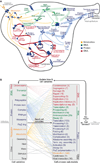
Figure 1. M. genitalium whole-cell model integrates 28 sub-models of diverse cellular processes
(A) Diagram schematically depicts the 28 sub-models as colored words – grouped by category as metabolic (orange), RNA (green), protein (blue), and DNA (red) – in the context of a single M. genitalium cell with its characteristic flask-like shape. Sub-models are connected through common metabolites, RNA, protein, and the chromosome which are depicted as orange, green, blue, and red colored arrows, respectively. (B) The model integrates cellular function sub-models through 16 cell state variables. First, simulations are randomly initialized to the beginning of the cell cycle (left grey arrow). Next, for each 1 s time step (dark black arrows) the sub-models retrieve the current values of the cellular variables, calculate their contributions to the temporal evolution of the cell variables, and update the values of the cellular variables. This is repeated thousands of times over the course of each simulation. For clarity, cell functions and variables are grouped into 5 physiologic categories: DNA (red), RNA (green), protein (blue), metabolite (orange), and other (black). Colored lines between the variables and sub-models indicate the cell variables predicted by each sub-model. The number of genes associated with each sub-model is indicated in parentheses. Finally, simulations are terminated upon cell division when the septum diameter equals zero (right grey arrow).
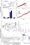
Figure 2. The model was trained with heterogeneous data and reproduces independent experimental data across multiple cellular functions and scales
(A) Growth of three cultures (dilutions indicated by shade of blue) and a blank control measured by OD550 of the pH indicator phenol red. The doubling time, τ, was calculated using the equation at the top left from the additional time required by more dilute cultures to reach the same OD550 (black lines). (B) Predicted growth dynamics of one life cycle of a population of 64 in silico cells (randomly chosen from the total simulation set). Median cell is highlighted in red. Distribution of cell cycle lengths is shown at bottom. (C) Comparison of the predicted and experimentally observed (Morowitz et al., 1962) cellular chemical compositions. Red bars indicate model s.d.; Morowitz et al. did not report s.d. (D) Temporal dynamics of the total cell mass and four cell mass fractions of a representative in silico cell. Mass fractions are normalized to their initial values. (E) Average predicted metabolic fluxes (see Figure S1B for metabolite and reaction labels). Arrow brightness indicates flux magnitude. The ratios of the GpsA and TalA fluxes to the Glk flux are indicated in orange boxes and are comparable to experimental data (Yus et al., 2009). (F) Ratios of observed (Sundararaj et al., 2004; Bennett et al., 2009) and average predicted concentrations of 39 metabolites. (G) Temporal dynamics of cytadherence high molecular weight protein 2 (HMW2, MG218) mRNA and protein expression of one in silico cell. Red dashed lines indicate the direct link between mRNA synthesis and subsequent bursts in protein synthesis. (H) HMW2 mRNA and protein copy number distribution of an unsynchronized population of 128 in silico cells. Histograms indicate the marginal distributions of the copy numbers of mRNA (top) and protein (right). Red lines indicate log-normal regressions of these marginal distributions. The absence of correlation between the copy numbers of mRNA and protein and the shapes of the marginal distributions are consistent with recent single-cell measurements by Taniguchi et al., 2010. See also Movie S1, and Tables S1 and S2.
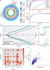
Figure 3. The model highlights the central physiologic role of DNA-protein interactions
(A) Average density of all DNA-bound proteins and of the replication initiation protein DnaA and DNA and RNA polymerase of a population of 128 in silico cells. Top magnification indicates the average density of DnaA at several sites near the oriC; DnaA forms a large multimeric complex at the sites indicated with asterisks, recruiting DNA polymerase to the oriC to initiate replication. Bottom left label indicates the location of the highly expressed rRNA genes. (B and C) Percentage of the chromosome that is predicted to have been bound (B), and the number of genes that are predicted to have been expressed (C) as functions of time. SMC is an abbreviated name for the name of the chromosome partition protein (MG298). (D) DNA-binding and dissociation dynamics of the oriC DnaA complex (red) and of RNA (blue) and DNA (green) polymerases for one in silico cell. The oriC DnaA complex recruits DNA polymerase to the oriC to initiate replication, which in turn dissolves the oriC DnaA complex. RNA polymerase traces (blue line segments) indicate individual transcription events. The height, length, and slope of each trace represent the transcript length, transcription duration, and transcript elongation rate, respectively. Inset highlights several predicted collisions between DNA and RNA polymerases leading to the displacement of RNA polymerases and incomplete transcripts.
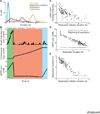
Figure 4. The model predictions regarding regulation of the cell cycle duration
(A) Distributions of the duration of three cell cycle phases, as well as that of the total cell cycle length, across 128 simulations. (B) Dynamics of macromolecule abundance in a selected cell simulation: top, the size of the DnaA complex assembling at the OriC (in monomers of DnaA); middle, the copy number of the chromosome; and bottom, the cytosolic dNTP concentration. The quantities of these macromolecules correlate strongly with the timing of key cell cycle stages. (C) Correlation between the initial cellular DnaA content and the duration of the replication initiation cell cycle stage across the same 128 in silico cells depicted in (A). (D) Correlation between the dNTP concentrations (both at the beginning of the cell cycle and at the beginning of replication) and the duration of replication across the same 128 in silico cells depicted in (A). (E) Correlation between the duration of replication initiation and replication across the same 128 in silico cells depicted in (A).
Figure 5. Model provides a global analysis of the use and allocation of energy
(A) Intracellular concentrations of the energy carriers ATP, GTP, FAD(H2), NAD(H), and NADP(H) of one in silico cell. (B) Comparison of the cell cycle length and total ATP and GTP usage of 128 in silico cells. (C) ATP (blue) and GTP (green) usage of 15 cellular processes throughout the life cycle of one in silico cell. The pie charts at right denote the percentage of ATP and GTP usage (red) as a fraction of total usage. (D) Average distribution of ATP and GTP usage among all modeled cellular processes in a population of 128 in silico cells. In total, the modeled processes account for only 44.3% of the amount of energy that has been experimentally observed to be produced during cellular growth.
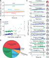
Figure 6. Model identifies common molecular pathologies underlying single-gene disruption phenotypes
(A) Comparison of predicted and observed (Glass et al., 2006) gene essentiality. Model predictions are based on at least five simulations of each single-gene disruption strain; see Data S1 for details. (B) Single-gene disruption strains were grouped into phenotypic classes (columns) according to their capacity to grow, synthesize protein, RNA, and DNA, and divide (indicated by septum length). Each column depicts the temporal dynamics of one representative in silico cell of each essential disruption strain class. Disruption strains of non-essential genes are not shown. Dynamics significantly different from wild type are highlighted in red. The identity of the representative cell and the number of disruption strains in each category is indicated in parenthesis. (C and D) Degradation and dilution of N-terminal protein content (C) of methionine aminopeptidase (map, MG172) disrupted cells causes reduced growth (D). Blue and black lines indicate the map disruption and wild type strains, respectively. Horizontal bars indicate s.d. See also Figure S2 for the distribution of simulated growth rates.
Figure 7. Quantitative characterization of selected gene disruption strains leads to identification of novel gene functions and kinetic parameters
(A) Comparison of measured and predicted growth rates for wild type and 12 single-gene disrupted strains. Model predictions that fall within the shaded region were considered consistent with experimental observations; the region has a width of four times the standard deviation of the wild type strain growth measurement. Error bars represent s.d. (B) Growth curves for the wild type and lpdA gene disruption strains and blank; similar to Figure 2A. (C) Expectation values determined by performing a pBLAST search of the M. genitalium genome with the LpdA sequence as a query. The asterisk and colored bar indicate a significant match (E < 10−6). (D) Detail of the M. genitalium genome. The pyruvate dehydrogenase complex genes are indicated by the top bracket, and transcription units identified in M. pneumoniae (Güell et al., 2009) are indicated by arrows. The transcription unit including nox is highlighted in color. (E) Allowing Nox to partially replace LpdA in pyruvate dehydrogenase reconciles model predictions and experimental observations. The blue and red lines represent the predicted wild type and Δ_lpdA_ strain growth rates as a function of the Nox-pyruvate dehydrogenase kcat. The pink box indicates the kcat at which the model predictions are consistent with both the wild type and Δ_lpdA_ strain experimentally measured growth rates. (F and G) Diagnosing the discrepancy between predictions and experiment for the thyA (F) and deoD (G) gene disruption strains. Some of the functionalities of ThyA and DeoD can be replaced by the enzymes Tdk and Pdp, respectively. The predicted growth rates of the wild type and gene disruption strains depend on the kcat of these enzymes. The green region highlights the range of kcat values consistent with the measured growth rates of both the wild type and gene disruption strain. (H) Newly predicted kcat values are similar to values that were measured in closely related organisms. Measured values of kcat for Tdk (top) and Pdp (bottom) are shown; green arrow indicates the initial and revised kcat values. The nearest M. genitalium relative is highlighted in green. (I) Model-based biological discovery. Comparison of model predictions to experimental measurements identified gene disruption strains of particular interest, including the lpdA, deoD and thyA disruption strains. Further investigation – using a combination of experiments, modeling and/or informatics – led to new and more consistent measurements and predictions. Most importantly, the higher consistency reflected novel insights into M. genitalium biology. The arrows (red for lpdA, green for deoD and thyA) indicate the shift from lower to higher consistency between model and experiment, and each arrow is annotated with the new biological insight and the supporting evidence in parentheses. The overall graph format is the same as Figure 7A.
Comment in
- The dawn of virtual cell biology.
Freddolino PL, Tavazoie S. Freddolino PL, et al. Cell. 2012 Jul 20;150(2):248-50. doi: 10.1016/j.cell.2012.07.001. Cell. 2012. PMID: 22817888 Free PMC article. - Silicon dreams of cells into symbols.
Gunawardena J. Gunawardena J. Nat Biotechnol. 2012 Sep;30(9):838-40. doi: 10.1038/nbt.2358. Nat Biotechnol. 2012. PMID: 22965055 No abstract available. - Life, simulated.
de Souza N. de Souza N. Nat Methods. 2012 Sep;9(9):861. doi: 10.1038/nmeth.2165. Nat Methods. 2012. PMID: 23097781 No abstract available.
Similar articles
- Accelerated discovery via a whole-cell model.
Sanghvi JC, Regot S, Carrasco S, Karr JR, Gutschow MV, Bolival B Jr, Covert MW. Sanghvi JC, et al. Nat Methods. 2013 Dec;10(12):1192-5. doi: 10.1038/nmeth.2724. Epub 2013 Nov 3. Nat Methods. 2013. PMID: 24185838 Free PMC article. - Systems biology: A cell in a computer.
Isalan M. Isalan M. Nature. 2012 Aug 2;488(7409):40-1. doi: 10.1038/488040a. Nature. 2012. PMID: 22859200 No abstract available. - Silicon dreams of cells into symbols.
Gunawardena J. Gunawardena J. Nat Biotechnol. 2012 Sep;30(9):838-40. doi: 10.1038/nbt.2358. Nat Biotechnol. 2012. PMID: 22965055 No abstract available. - The Unique Microbiology and Molecular Pathogenesis of Mycoplasma genitalium.
McGowin CL, Totten PA. McGowin CL, et al. J Infect Dis. 2017 Jul 15;216(suppl_2):S382-S388. doi: 10.1093/infdis/jix172. J Infect Dis. 2017. PMID: 28838077 Free PMC article. Review. - Mycoplasma genitalium: a significant urogenital pathogen ?
Ekiel A, Jóźwiak J, Martirosian G. Ekiel A, et al. Med Sci Monit. 2009 Apr;15(4):RA102-6. Med Sci Monit. 2009. PMID: 19333215 Review.
Cited by
- From integrative structural biology to cell biology.
Sali A. Sali A. J Biol Chem. 2021 Jan-Jun;296:100743. doi: 10.1016/j.jbc.2021.100743. Epub 2021 May 4. J Biol Chem. 2021. PMID: 33957123 Free PMC article. Review. - Invariance and optimality in the regulation of an enzyme.
Reznik E, Yohe S, Segrè D. Reznik E, et al. Biol Direct. 2013 Mar 22;8:7. doi: 10.1186/1745-6150-8-7. Biol Direct. 2013. PMID: 23522082 Free PMC article. - History and Future Perspectives on the Discipline of Quantitative Systems Pharmacology Modeling and Its Applications.
Azer K, Kaddi CD, Barrett JS, Bai JPF, McQuade ST, Merrill NJ, Piccoli B, Neves-Zaph S, Marchetti L, Lombardo R, Parolo S, Immanuel SRC, Baliga NS. Azer K, et al. Front Physiol. 2021 Mar 25;12:637999. doi: 10.3389/fphys.2021.637999. eCollection 2021. Front Physiol. 2021. PMID: 33841175 Free PMC article. Review. - The analysis of living systems can generate both knowledge and illusions.
Jose AM. Jose AM. Elife. 2020 Jun 18;9:e56354. doi: 10.7554/eLife.56354. Elife. 2020. PMID: 32553111 Free PMC article. - Potential unsatisfiability of cyclic constraints on stochastic biological networks biases selection towards hierarchical architectures.
Smith C, Pechuan X, Puzio RS, Biro D, Bergman A. Smith C, et al. J R Soc Interface. 2015 Jul 6;12(108):20150179. doi: 10.1098/rsif.2015.0179. J R Soc Interface. 2015. PMID: 26040595 Free PMC article.
References
- Atlas JC, Nikolaev EV, Browning ST, Shuler ML. Incorporating genome-wide DNA sequence information into a dynamic whole-cell model of Escherichia coli: application to DNA replication. IET Syst. Biol. 2008;2:369–382. - PubMed
- Browning ST, Castellanos M, Shuler ML. Robust control of initiation of prokaryotic chromosome replication: essential considerations for a minimal cell. Biotechnol. Bioeng. 2004;88:575–584. - PubMed
Publication types
MeSH terms
Substances
LinkOut - more resources
Full Text Sources
Other Literature Sources
