Stacks: an analysis tool set for population genomics - PubMed (original) (raw)
. 2013 Jun;22(11):3124-40.
doi: 10.1111/mec.12354. Epub 2013 May 24.
Affiliations
- PMID: 23701397
- PMCID: PMC3936987
- DOI: 10.1111/mec.12354
Stacks: an analysis tool set for population genomics
Julian Catchen et al. Mol Ecol. 2013 Jun.
Abstract
Massively parallel short-read sequencing technologies, coupled with powerful software platforms, are enabling investigators to analyse tens of thousands of genetic markers. This wealth of data is rapidly expanding and allowing biological questions to be addressed with unprecedented scope and precision. The sizes of the data sets are now posing significant data processing and analysis challenges. Here we describe an extension of the Stacks software package to efficiently use genotype-by-sequencing data for studies of populations of organisms. Stacks now produces core population genomic summary statistics and SNP-by-SNP statistical tests. These statistics can be analysed across a reference genome using a smoothed sliding window. Stacks also now provides several output formats for several commonly used downstream analysis packages. The expanded population genomics functions in Stacks will make it a useful tool to harness the newest generation of massively parallel genotyping data for ecological and evolutionary genetics.
© 2013 John Wiley & Sons Ltd.
Figures
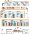
Fig. 1
The Stacks pipeline. Stacks proceeds in five major stages. First, reads are demultiplexed and cleaned by the process_rad-tags program. The next three stages comprise the main Stacks pipeline: building loci (ustacks/pstacks), creating the catalogue of loci (cstacks) and matching against the catalogue (sstacks). In the fifth stage, either the populations or genotypes program is executed, depending on the type of input data. The populations program tabulates the state of loci within and among populations, calculates population genetics statistics and exports to a number of additional, useful formats. The genotypes program is further described in Catchen et al. 2011.
Fig. 2
The ustacks deleveraging algorithm. (A) The simplest polymorphic locus is defined by a single SNP (A/T), and as the remainder of the locus is identical in both alleles, we can refer to the entire locus by the A/T haplotypes. A locus can be visualized as an undirected graph, with each allele or stack as a node, and with the nodes connected by an edge weighted according to the nucleotide distance between them. (B) This locus with three detected polymorphisms comprises six distinct stacks, which is not biologically possible and must be the result of either erroneous stacks or collapsed, repetitive loci. The deleveraging algorithm calculates a minimum-spanning tree from the locus (thick, black lines), calculates the minimum distance between any two nodes and breaks edges (separating loci) whenever they are connected by edges larger than the minimum edge. The result in this case is two loci, the first built from stacks 0, 1 and 2, and the second built from stacks 3, 4 and 5.
Fig. 3
The bounded-error SNP calling model. Curves show log likelihood of the two most likely genotypes (homozygote 1/1 or heterozygote 1/2) as a function of sequencing error rate ε. In this example, n1 = 8, n2 = 2 and n3 = 1 (the constant resulting from the multinomial coefficient is the same for each genotype and is omitted from the calculation). If ε is unbounded, the likelihood of each genotype is calculated at the maximum-likelihood estimate of ε (solid horizontal lines), homozygote is most likely, and a likelihood ratio test depends on the difference between the two log likelihoods (upper curved brace). If ε is bounded above by 0.1 (dashed vertical line), the likelihood of each genotype is calculated for the Maximum Likelihood Estimator of ε within this interval (dashed horizontal lines), and in this case, heterozygote is now the most likely genotype.
Fig. 4
Kernel-smoothing algorithm. Stacks’s populations program can generate a kernel-smoothed moving average across each contig, scaffold or chromosome by applying a Gaussian weighting function (inset formula, the red curves show how highly weighted each nucleotide position in the window will be). For each population, the sliding window is centred over each polymorphic locus, C/G, T/C and A/T, in this example. At each locus, weights are generated by the Gaussian function for all the measures of either _F_IS or π within the window to generate a smoothed average from that window. The size of the window is determined by σ, and by default, the tail of each side of the window is truncated at 3σ base pair. This algorithm is also applied to pairs of populations to generate a kernel-smoothed _F_ST measure in the same manner.
Fig. 5
De novo stack formation. (A) We ran ustacks against 590 threespine stickleback fish and compared these de novo results against the same data set aligned against the threespine stickleback reference genome. On average, 37 184.6 de novo loci aligned to a single location in the reference indicating they were correctly constructed. A small number of loci align to multiple places in the genome indicating incorrect de novo construction. (B–D) We explored how three key parameters affect the formation of de novo loci. (B) Allowing two mismatches between stacks (equivalent to nucleotide distance) results in 990 de novo loci that should be merged into 492 loci according to the reference genome. Increasing -M reduces these undermerged loci, although the rate of reduction decreases after -M 4. (C) As we increase the minimum number of raw reads required to form a stack, we see a trade-off between the number of false loci removed from our data set (blue line) vs. the number of true loci lost due to low coverage of the locus (green line). (D) As we increase the number of stacks allowed to exist at a single locus, we see a trade-off between the number of true loci added to the data set (green line) vs. the number of collapsed, false loci we add to the data set (blue line).
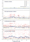
Fig. 6
Kernel-smoothed _F_ST analysis. A comparison of four populations of Oregon threespine stickleback spanning a range of geographical distances using _F_ST scans from the Stacks populations program. (A) The two marine populations, which are phenotypically similar and geographically close, show no significant divergence along linkage group I. (B) The coastal fresh and marine populations show clusters of highly significantly diverged SNPs from 7 to 12 Mb of group I. (C) In the marine by Willamette basin comparison, a series of divergent SNPs raise the overall level of _F_ST along the entire chromosome and probably represent neutral differences accumulated during the long separation of the populations. (D) The large number of fixed differences SNPs with an _F_ST of 1.0) in comparison between marine and central Oregon fish is the result of genetic sub-sampling during recent founding of the inland populations.
Similar articles
- Stacks 2: Analytical methods for paired-end sequencing improve RADseq-based population genomics.
Rochette NC, Rivera-Colón AG, Catchen JM. Rochette NC, et al. Mol Ecol. 2019 Nov;28(21):4737-4754. doi: 10.1111/mec.15253. Epub 2019 Oct 17. Mol Ecol. 2019. PMID: 31550391 - Population genomic analysis of model and nonmodel organisms using sequenced RAD tags.
Hohenlohe PA, Catchen J, Cresko WA. Hohenlohe PA, et al. Methods Mol Biol. 2012;888:235-60. doi: 10.1007/978-1-61779-870-2_14. Methods Mol Biol. 2012. PMID: 22665285 - From reference genomes to population genomics: comparing three reference-aligned reduced-representation sequencing pipelines in two wildlife species.
Wright B, Farquharson KA, McLennan EA, Belov K, Hogg CJ, Grueber CE. Wright B, et al. BMC Genomics. 2019 Jun 3;20(1):453. doi: 10.1186/s12864-019-5806-y. BMC Genomics. 2019. PMID: 31159724 Free PMC article. - Sequencing pools of individuals - mining genome-wide polymorphism data without big funding.
Schlötterer C, Tobler R, Kofler R, Nolte V. Schlötterer C, et al. Nat Rev Genet. 2014 Nov;15(11):749-63. doi: 10.1038/nrg3803. Epub 2014 Sep 23. Nat Rev Genet. 2014. PMID: 25246196 Review. - Harnessing the power of RADseq for ecological and evolutionary genomics.
Andrews KR, Good JM, Miller MR, Luikart G, Hohenlohe PA. Andrews KR, et al. Nat Rev Genet. 2016 Feb;17(2):81-92. doi: 10.1038/nrg.2015.28. Epub 2016 Jan 5. Nat Rev Genet. 2016. PMID: 26729255 Free PMC article. Review.
Cited by
- An endangered flightless grasshopper with strong genetic structure maintains population genetic variation despite extensive habitat loss.
Hoffmann AA, White VL, Jasper M, Yagui H, Sinclair SJ, Kearney MR. Hoffmann AA, et al. Ecol Evol. 2021 Apr 4;11(10):5364-5380. doi: 10.1002/ece3.7428. eCollection 2021 May. Ecol Evol. 2021. PMID: 34026013 Free PMC article. - Identifying the fitness costs of a pyrethroid-resistant genotype in the major arboviral vector Aedes aegypti.
Rigby LM, Rašić G, Peatey CL, Hugo LE, Beebe NW, Devine GJ. Rigby LM, et al. Parasit Vectors. 2020 Jul 20;13(1):358. doi: 10.1186/s13071-020-04238-4. Parasit Vectors. 2020. PMID: 32690061 Free PMC article. - Landscape genomics reveals genetic signals of environmental adaptation of African wild eggplants.
Omondi EO, Lin CY, Huang SM, Liao CA, Lin YP, Oliva R, van Zonneveld M. Omondi EO, et al. Ecol Evol. 2024 Jul 9;14(7):e11662. doi: 10.1002/ece3.11662. eCollection 2024 Jul. Ecol Evol. 2024. PMID: 38983700 Free PMC article. - Species distribution models predict genetic isolation of Hetaerina vulnerata Hagen in Selys, 1853 (Odonata, Calopterygidae).
Biddy AR, Manthey JD, Ware JL, McIntyre NE. Biddy AR, et al. Ecol Evol. 2024 Aug 6;14(8):e70107. doi: 10.1002/ece3.70107. eCollection 2024 Aug. Ecol Evol. 2024. PMID: 39108563 Free PMC article. - Phylogeographic and population genetic analyses reveal multiple species of Boa and independent origins of insular dwarfism.
Card DC, Schield DR, Adams RH, Corbin AB, Perry BW, Andrew AL, Pasquesi GI, Smith EN, Jezkova T, Boback SM, Booth W, Castoe TA. Card DC, et al. Mol Phylogenet Evol. 2016 Sep;102:104-16. doi: 10.1016/j.ympev.2016.05.034. Epub 2016 May 27. Mol Phylogenet Evol. 2016. PMID: 27241629 Free PMC article.
References
- Amish SJ, Hohenlohe PA, Painter S, et al. RAD sequencing yields a high success rate for westslope cutthroat and rainbow trout species-diagnostic SNP assays. Molecular Ecology Resources. 2012;12:653–660. - PubMed
- Andrew RL, Kane NC, Baute GJ, Grassa CJ, Rieseberg LH. Recent nonhybrid origin of sunflower ecotypes in a novel habitat. Molecular Ecology. 2013;22:799–813. - PubMed
Publication types
MeSH terms
Substances
Grants and funding
- P30 GM103324/GM/NIGMS NIH HHS/United States
- R24 OD011199/OD/NIH HHS/United States
- R24 GM079486/GM/NIGMS NIH HHS/United States
- P20RR16448/RR/NCRR NIH HHS/United States
- R24 RR032670/RR/NCRR NIH HHS/United States
- 1R24GM079486-01A1/GM/NIGMS NIH HHS/United States
- F32GM095213-01/GM/NIGMS NIH HHS/United States
- P20 RR016448/RR/NCRR NIH HHS/United States
- F32 GM095213/GM/NIGMS NIH HHS/United States
LinkOut - more resources
Full Text Sources
Other Literature Sources
Molecular Biology Databases


