A double-edged sword: Benefits and pitfalls of heterogeneous punishment in evolutionary inspection games - PubMed (original) (raw)
A double-edged sword: Benefits and pitfalls of heterogeneous punishment in evolutionary inspection games
Matjaž Perc et al. Sci Rep. 2015.
Abstract
As a simple model for criminal behavior, the traditional two-strategy inspection game yields counterintuitive results that fail to describe empirical data. The latter shows that crime is often recurrent, and that crime rates do not respond linearly to mitigation attempts. A more apt model entails ordinary people who neither commit nor sanction crime as the third strategy besides the criminals and punishers. Since ordinary people free-ride on the sanctioning efforts of punishers, they may introduce cyclic dominance that enables the coexistence of all three competing strategies. In this setup ordinary individuals become the biggest impediment to crime abatement. We therefore also consider heterogeneous punisher strategies, which seek to reduce their investment into fighting crime in order to attain a more competitive payoff. We show that this diversity of punishment leads to an explosion of complexity in the system, where the benefits and pitfalls of criminal behavior are revealed in the most unexpected ways. Due to the raise and fall of different alliances no less than six consecutive phase transitions occur in dependence on solely the temptation to succumb to criminal behavior, leading the population from ordinary people-dominated across punisher-dominated to crime-dominated phases, yet always failing to abolish crime completely.
Figures
Figure 1. Phase diagram of the three-strategy spatial inspection game with uniform punishment.
Depicted are strategies remaining on the square lattice after sufficiently long relaxation times as a function of the temptation/loss β and the reward for punishing criminals γ, as obtained for the the punishment cost α = 0.5. Here C marks the parameter region where the population terminates in a homogeneous “all-criminal” phase, C + P marks the region where criminals and punishers coexist, while in the O + C + P region all three strategies are present in the stationary state due to cyclic dominance. Solid blue lines denote continuous phase transitions, while the dashed red line denotes the border of cyclic dominance between competing strategies.
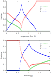
Figure 2. Two characteristic cross-sections of the phase diagram depicted in Fig. 1.
Left panel shows the fraction of the three strategies in dependence on the temptation/loss β at γ = 0.8. Starting at the three-strategy O + C + P phase, the fraction of ordinary people and the criminals decreases steadily with increasing the value of β until eventually O die out and the two-strategy C + P phase is reached. Immediately thereafter the fraction of criminals starts rising as the value of β increases further, with the second continuous phase transition marking the emergence of the pure C phase. Right panel shows the fraction of the three strategies in dependence on the reward for punishing criminals γ at β = 0.8. In this case we start at the pure C phase, which turns to the two-strategy C + P phase as soon as γ is large enough to sustain the punishers. As γ increases further ordinary people become viable too through a second continuous phase transition, ultimately yielding the three-strategy O + C + P phase that is maintained by cyclic dominance. In both panels the punishment cost is α = 0.5.
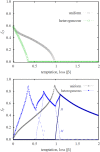
Figure 3. Left panel shows the fraction of ordinary people in dependence on the temptation/loss β, as obtained for the three-strategy spatial inspection game with uniform punishment and the five-strategy spatial inspection game with heterogeneous punishment (see legend).
It can be observed that heterogeneous punishment is indeed more effective in eliminating second-order free-riding by ordinary people than uniform punishment. Right panel shows the fraction of punishers in dependence on the temptation/loss β for the uniform punishment model and the aggregate fraction of all punishers in the heterogeneous punishment model, as well as the fraction of punishers L, M and H individually (see legend). The success of heterogeneous punishment to eliminate second-order free-riding is somewhat relativized, as higher punishment levels will not necessarily lead to lower criminal levels (see Fig. 4 for an explanation). The origin of the zig-zag outlay of the aggregate fraction of all punishers is analyzed in Fig. 5. In both panels the punishment cost is α = 0.5 and the reward for punishing criminals is γ = 1.5.
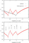
Figure 4. Top panel shows the fraction of criminals in dependence on the temptation/loss β, as obtained for the three-strategy spatial inspection game with uniform punishment and the five-strategy spatial inspection game with heterogeneous punishment (see legend).
It can be observed that heterogeneous punishment is more effective than uniform punishment in eliminating crime only in the low β limit, which also agrees with the region in which second-order free-riding is deterred more efficiently (see Fig. 3). In general, however, uniform punishment works just as well or better than heterogeneous punishment in abating crime. Bottom panel again shows the fraction of criminals, along with the different phases that contain the C strategy. Despite the multitude of consecutive phase transitions in dependence on solely a single parameter, criminal behavior is never completely eliminated. In both panels the punishment cost is α = 0.5 and the reward for punishing criminals is γ = 1.5.
Figure 5. Time evolution of strategy distributions in the population, as obtained with the heterogeneous punishment game starting from the same prepared initial state (leftmost panel) for γ = 1.5 and three different values of the temptation/loss.
(a)–(d) β = 0.5, (e)–(h) β = 0.9, and (i)–(l) β = 0.7. The resulting three different stationary states are reached within 400 MCS, which are depicted in the rightmost panels. Colors red, light blue and dark blue depict the location of C, L and M players, respectively. For visual clarity, we have used a small 150 × 150 system size. See main text for a detailed description of the different evolutionary outcomes.
Similar articles
- Understanding recurrent crime as system-immanent collective behavior.
Perc M, Donnay K, Helbing D. Perc M, et al. PLoS One. 2013 Oct 4;8(10):e76063. doi: 10.1371/journal.pone.0076063. eCollection 2013. PLoS One. 2013. PMID: 24124533 Free PMC article. - Recidivism and rehabilitation of criminal offenders: a carrot and stick evolutionary game.
Berenji B, Chou T, D'Orsogna MR. Berenji B, et al. PLoS One. 2014 Jan 16;9(1):e85531. doi: 10.1371/journal.pone.0085531. eCollection 2014. PLoS One. 2014. PMID: 24454884 Free PMC article. - Phase diagrams for the spatial public goods game with pool punishment.
Szolnoki A, Szabó G, Perc M. Szolnoki A, et al. Phys Rev E Stat Nonlin Soft Matter Phys. 2011 Mar;83(3 Pt 2):036101. doi: 10.1103/PhysRevE.83.036101. Epub 2011 Mar 7. Phys Rev E Stat Nonlin Soft Matter Phys. 2011. PMID: 21517552 - Symbiotic behaviour in the public goods game with altruistic punishment.
Flores LS, Fernandes HCM, Amaral MA, Vainstein MH. Flores LS, et al. J Theor Biol. 2021 Sep 7;524:110737. doi: 10.1016/j.jtbi.2021.110737. Epub 2021 Apr 28. J Theor Biol. 2021. PMID: 33930439 - Individual mobility promotes punishment in evolutionary public goods games.
Cong R, Zhao Q, Li K, Wang L. Cong R, et al. Sci Rep. 2017 Oct 25;7(1):14015. doi: 10.1038/s41598-017-12823-4. Sci Rep. 2017. PMID: 29070844 Free PMC article.
Cited by
- Criminal organizations exhibit hysteresis, resilience, and robustness by balancing security and efficiency.
van Elteren C, Vasconcelos VV, Lees M. van Elteren C, et al. Sci Rep. 2024 Jul 30;14(1):17678. doi: 10.1038/s41598-024-68445-0. Sci Rep. 2024. PMID: 39085455 Free PMC article. - Environmental Governance Cooperative Behavior among Enterprises with Reputation Effect Based on Complex Networks Evolutionary Game Model.
Luo M, Fan R, Zhang Y, Zhu C. Luo M, et al. Int J Environ Res Public Health. 2020 Feb 27;17(5):1535. doi: 10.3390/ijerph17051535. Int J Environ Res Public Health. 2020. PMID: 32120950 Free PMC article. - Environment-based preference selection promotes cooperation in spatial prisoner's dilemma game.
Wu Y, Zhang S, Zhang Z. Wu Y, et al. Sci Rep. 2018 Oct 23;8(1):15616. doi: 10.1038/s41598-018-34116-0. Sci Rep. 2018. PMID: 30353150 Free PMC article. - Strategy intervention for the evolution of fairness.
Zhang Y, Fu F. Zhang Y, et al. PLoS One. 2018 May 2;13(5):e0196524. doi: 10.1371/journal.pone.0196524. eCollection 2018. PLoS One. 2018. PMID: 29718977 Free PMC article. - The probabilistic pool punishment proportional to the difference of payoff outperforms previous pool and peer punishment.
Ohdaira T. Ohdaira T. Sci Rep. 2022 Apr 22;12(1):6604. doi: 10.1038/s41598-022-10582-5. Sci Rep. 2022. PMID: 35459880 Free PMC article.
References
- Wilson J. Q. & Kelling G. L. Broken windows. The Atlantic Monthly 249, 29–38 (1982).
- Rigney D. The Matthew effect: How advantage begets further advantage (Columbia University Press, New York, 2013).
- Barabási A.-L. & Albert R. Emergence of scaling in random networks. Science 286, 509–512 (1999). - PubMed
- Albert R. & Barabási A. L. Statistical mechanics of complex networks. Rev. Mod. Phys. 74, 47–97 (2002).
MeSH terms
LinkOut - more resources
Full Text Sources
Other Literature Sources
Research Materials


