The fallacy of placing confidence in confidence intervals - PubMed (original) (raw)
The fallacy of placing confidence in confidence intervals
Richard D Morey et al. Psychon Bull Rev. 2016 Feb.
Abstract
Interval estimates - estimates of parameters that include an allowance for sampling uncertainty - have long been touted as a key component of statistical analyses. There are several kinds of interval estimates, but the most popular are confidence intervals (CIs): intervals that contain the true parameter value in some known proportion of repeated samples, on average. The width of confidence intervals is thought to index the precision of an estimate; CIs are thought to be a guide to which parameter values are plausible or reasonable; and the confidence coefficient of the interval (e.g., 95 %) is thought to index the plausibility that the true parameter is included in the interval. We show in a number of examples that CIs do not necessarily have any of these properties, and can lead to unjustified or arbitrary inferences. For this reason, we caution against relying upon confidence interval theory to justify interval estimates, and suggest that other theories of interval estimation should be used instead.
Keywords: Bayesian inference and parameter estimation; Bayesian statistics; Statistical inference; Statistics.
Figures
Fig. 1
Submersible rescue attempts. Note that likelihood and CIs are depicted from bottom to top in the order in which they are described in the text. See text for details. An interactive version of this figure is available at
http://learnbayes.org/redirects/CIshiny1.html
Fig. 2
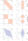
Left: Possible locations of the first (y 1) and second (y 2) bubbles. Right: y 2−y 1 plotted against the mean of y 1 and y 2. Shaded regions show the areas where the respective 50 % confidence interval contains the true value. The figures in the top row (a, b) show the sampling distribution interval; the middle row (c, d) shows the NP and UMP intervals; the bottom row (e, f) shows the Bayes interval. Points ‘a’ and ‘b’ represent the pairs of bubbles from Fig. 1a and b, respectively. An interactive version of this figure is available at
http://learnbayes.org/redirects/CIshiny1.html
Fig. 3
The relationship between CI width and the uncertainty in the estimation of the hatch location for the four confidence procedures. SD: Sampling distribution procedure; NP: Nonparametric procedure; UMP: UMP procedure; B: Bayes procedure. Note that the NP and UMP procedures overlap when the width of the likelihood is >5. An interactive version of this figure is available at
http://learnbayes.org/redirects/CIshiny1.html
Fig. 4
The probability that each confidence procedure includes false values 𝜃′. T: Trivial procedure; SD: Sampling distribution procedure NP: Nonparametric procedure; UMP: UMP procedure; B: Bayes procedure. The line for the sampling distribution procedure (dashed line) is between the lines for the Bayes procedure and the UMP procedure. An interactive version of this figure is available at
http://learnbayes.org/redirects/CIshiny1.html
Fig. 5
Forming Bayesian credible intervals. Prior information (top) is combined with the likelihood information from the data (middle) to yield a posterior distribution (bottom). In the likelihood plots, the shaded regions show the locations within 5 meters of each bubble; the dark shaded regions show where these overlap, indicating the possible location of the hatch θ. In the posterior plots, the central 50 % region (shaded region within posterior) shows one possible 50 % credible interval, the central credible interval. An interactive version of this figure is available at
http://learnbayes.org/redirects/CIshiny1.html
Fig. 6
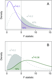
Building a confidence interval by inverting a significance test. A: Two noncentral F distributions, with true ω 2 = .1 (blue solid line) and true ω 2 = .2 (dashed gray line). When F(2,27)=5, the upper-tailed p value for these tests are .16 and .42, respectively. B: Two noncentral F distributions, with true ω 2 = .36 (red solid line) and true ω 2 = .2 (dashed gray line). When F(2,27)=5, the lower-tailed p value for these tests are .16 and .58, respectively
Fig. 7
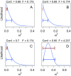
Likelihoods, confidence intervals, and Bayesian credible intervals (highest posterior density, or HPD, intervals) for four hypothetical experimental results. In each figure, the top interval is Steiger’s (2004) confidence interval for ω 2; the bottom interval is the Bayesian HPD. See text for details
Similar articles
- Understanding and interpreting confidence and credible intervals around effect estimates.
Hespanhol L, Vallio CS, Costa LM, Saragiotto BT. Hespanhol L, et al. Braz J Phys Ther. 2019 Jul-Aug;23(4):290-301. doi: 10.1016/j.bjpt.2018.12.006. Epub 2018 Dec 31. Braz J Phys Ther. 2019. PMID: 30638956 Free PMC article. Review. - Empirical Bayes interval estimates that are conditionally equal to unadjusted confidence intervals or to default prior credibility intervals.
Bickel DR. Bickel DR. Stat Appl Genet Mol Biol. 2012 Feb 21;11(3):Article 7. doi: 10.1515/1544-6115.1765. Stat Appl Genet Mol Biol. 2012. PMID: 22499708 - Accurate Confidence and Bayesian Interval Estimation for Non-centrality Parameters and Effect Size Indices.
Kang K, Jones MT, Armstrong K, Avery S, McHugo M, Heckers S, Vandekar S. Kang K, et al. Psychometrika. 2023 Mar;88(1):253-273. doi: 10.1007/s11336-022-09899-x. Epub 2023 Feb 1. Psychometrika. 2023. PMID: 36725775 Free PMC article. - Applications of Monte Carlo Simulation in Modelling of Biochemical Processes.
Tenekedjiev KI, Nikolova ND, Kolev K. Tenekedjiev KI, et al. In: Mode CJ, editor. Applications of Monte Carlo Methods in Biology, Medicine and Other Fields of Science [Internet]. Rijeka (HR): InTech; 2011 Feb 28. Chapter 4. In: Mode CJ, editor. Applications of Monte Carlo Methods in Biology, Medicine and Other Fields of Science [Internet]. Rijeka (HR): InTech; 2011 Feb 28. Chapter 4. PMID: 28045483 Free Books & Documents. Review.
Cited by
- Applied Bayesian Approaches for Research in Motor Neuron Disease.
Temp AGM, Naumann M, Hermann A, Glaß H. Temp AGM, et al. Front Neurol. 2022 Mar 24;13:796777. doi: 10.3389/fneur.2022.796777. eCollection 2022. Front Neurol. 2022. PMID: 35401404 Free PMC article. - Concise, Simple, and Not Wrong: In Search of a Short-Hand Interpretation of Statistical Significance.
Spence JR, Stanley DJ. Spence JR, et al. Front Psychol. 2018 Nov 13;9:2185. doi: 10.3389/fpsyg.2018.02185. eCollection 2018. Front Psychol. 2018. PMID: 30483192 Free PMC article. - Identifying Links Between Latent Memory and Speech Recognition Factors.
Bosen AK, Doria GM. Bosen AK, et al. Ear Hear. 2024 Mar-Apr 01;45(2):351-369. doi: 10.1097/AUD.0000000000001430. Epub 2023 Oct 26. Ear Hear. 2024. PMID: 37882100 Free PMC article. - Agile software development one year into the COVID-19 pandemic.
Ågren P, Knoph E, Berntsson Svensson R. Ågren P, et al. Empir Softw Eng. 2022;27(6):121. doi: 10.1007/s10664-022-10176-9. Epub 2022 Jun 22. Empir Softw Eng. 2022. PMID: 35757145 Free PMC article. - The reporting of p values, confidence intervals and statistical significance in Preventive Veterinary Medicine (1997-2017).
Messam LLM, Weng HY, Rosenberger NWY, Tan ZH, Payet SDM, Santbakshsing M. Messam LLM, et al. PeerJ. 2021 Nov 24;9:e12453. doi: 10.7717/peerj.12453. eCollection 2021. PeerJ. 2021. PMID: 34900418 Free PMC article.
References
- Anastasi A, Urbina S. Psychological testing. 7th ed. London: Prentice-Hall International; 1997.
- Basu D. On ancillary statistics, pivotal quantities, and confidence statements. In: Chaubey Y P, Dwivedi T D, editors. Topics in applied statistics. Montreal: Concordia University; 1981. pp. 1–29.
- Berger JO. Bayes factors. In: Kotz S, Balakrishnan N, Read C, Vidakovic B, Johnson N L, editors. Encyclopedia of statistical sciences (Second edition) Hoboken, New Jersey: John Wiley & Sons; 2006. pp. 378–386.
- Berger JO, Wolpert RL. The likelihood principle (2nd ed.) Hayward. CA: Institute of Mathematical Statistics; 1988.
- Blaker H, Spjøtvoll E. Paradoxes and improvements in interval estimation. The American Statistician. 2000;54(4):242–247.
Publication types
MeSH terms
LinkOut - more resources
Full Text Sources
Other Literature Sources


