Genome graphs and the evolution of genome inference - PubMed (original) (raw)
Review
Genome graphs and the evolution of genome inference
Benedict Paten et al. Genome Res. 2017 May.
Abstract
The human reference genome is part of the foundation of modern human biology and a monumental scientific achievement. However, because it excludes a great deal of common human variation, it introduces a pervasive reference bias into the field of human genomics. To reduce this bias, it makes sense to draw on representative collections of human genomes, brought together into reference cohorts. There are a number of techniques to represent and organize data gleaned from these cohorts, many using ideas implicitly or explicitly borrowed from graph-based models. Here, we survey various projects underway to build and apply these graph-based structures-which we collectively refer to as genome graphs-and discuss the improvements in read mapping, variant calling, and haplotype determination that genome graphs are expected to produce.
© 2017 Paten et al.; Published by Cold Spring Harbor Laboratory Press.
Figures
Figure 1.
Schematic representation of two population-level reference structures. (A) A reference cohort, in which there is no attempt to identify homologies between the genome sequences. (B) A genome graph, in which homologies are collapsed and included as alternate paths in the graph.
Figure 2.
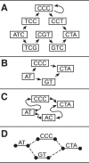
Four types of genome graphs, all constructed from the pair of sequences
ATCCCCTA
and
ATGTCTA
. (A) De Bruijn graph. (B) Directed acyclic graph. (C) Bidirected graph (a.k.a., sequence graph). (D) Biedged graph (a.k.a., biedged sequence graph).
Figure 3.
Ultrabubble sites in a biedged sequence graph. Each arrow shows the terminal node of a site. The color of the arrows indicates the node pairing. Note that the ultrabubble denoted by the gray pair of arrows is nested within the ultrabubble denoted by the purple arrows. (Reprinted from Paten et al. 2017, with permission from the author.)
Figure 4.
A pangenome ordering on a graph constructed from two genomes. The red edges indicate the path of the pangenome through the graph. The solid and dotted edges indicate the adjacencies between nodes in the two source genomes. (Adapted from Nguyen et al. 2015, with permission from the author.)
Figure 5.
A schematic example of an “Array Sequence Graph” of the type used to construct a linearization of the DXZ1 repeat array in the X Chromosome centromere (Miga et al. 2014). A collection of reads (top) shown in the context of a consensus higher-order repeat are converted into a graph representation (bottom). A cycle around the graph represents a higher-order repeat, and the individual repeat units (oblongs) are represented within each node (circles). Edges between individual repeat units represent phasing information from input reads. Transitions between nodes are annotated with probabilities. (Adapted from Miga et al. 2014, with permission from the author.)
Figure 6.
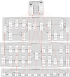
A reference genome graph hierarchy (most collapsed graph at the top, less collapsed lower), with an input graph (bottom) mapped to it. All the graphs in the reference hierarchy are de Bruijn graphs. Dotted red lines show projections between graphs in the hierarchy, whereas solid red lines show mapping of the input sequence graph into the hierarchy. Here, each node has a unique ID, and the L and R strings represent flanking contexts mapping strings required for unique identification. (Reprinted from Paten et al. 2014, with permission from the author.)
Figure 7.
Distinct 1000 Genomes Project haplotypes embedded within a variation subgraph. Haplotypes are shown as colored ribbons with width proportional to the log of their frequency. The number of possible paths traversing left to right is 16, but only five are observed in the 1000 Genomes Project because of linkage disequilibrium. (Figure based on prototype by W Beyer, pers. comm.)
Figure 8.
Bidirected sequence graph (A) being unfolded into a directed acyclic graph (B), in preparation for partial-order alignment. Node 6 is a reversed view of node 1, node 7 is a reversed view of node 2, and node 8 is a reversed view of node 5. (Reprinted from Garrison et al. [in prep], with permission from the author.)
Similar articles
- Fast and accurate genomic analyses using genome graphs.
Rakocevic G, Semenyuk V, Lee WP, Spencer J, Browning J, Johnson IJ, Arsenijevic V, Nadj J, Ghose K, Suciu MC, Ji SG, Demir G, Li L, Toptaş BÇ, Dolgoborodov A, Pollex B, Spulber I, Glotova I, Kómár P, Stachyra AL, Li Y, Popovic M, Källberg M, Jain A, Kural D. Rakocevic G, et al. Nat Genet. 2019 Feb;51(2):354-362. doi: 10.1038/s41588-018-0316-4. Epub 2019 Jan 14. Nat Genet. 2019. PMID: 30643257 - Positional bias in variant calls against draft reference assemblies.
Briskine RV, Shimizu KK. Briskine RV, et al. BMC Genomics. 2017 Mar 28;18(1):263. doi: 10.1186/s12864-017-3637-2. BMC Genomics. 2017. PMID: 28351369 Free PMC article. - Pan-African genome demonstrates how population-specific genome graphs improve high-throughput sequencing data analysis.
Tetikol HS, Turgut D, Narci K, Budak G, Kalay O, Arslan E, Demirkaya-Budak S, Dolgoborodov A, Kabakci-Zorlu D, Semenyuk V, Jain A, Davis-Dusenbery BN. Tetikol HS, et al. Nat Commun. 2022 Aug 4;13(1):4384. doi: 10.1038/s41467-022-31724-3. Nat Commun. 2022. PMID: 35927245 Free PMC article. - Pangenome graphs and their applications in biodiversity genomics.
Secomandi S, Gallo GR, Rossi R, Rodríguez Fernandes C, Jarvis ED, Bonisoli-Alquati A, Gianfranceschi L, Formenti G. Secomandi S, et al. Nat Genet. 2025 Jan;57(1):13-26. doi: 10.1038/s41588-024-02029-6. Epub 2025 Jan 8. Nat Genet. 2025. PMID: 39779953 Review. - Pangenome Graphs.
Eizenga JM, Novak AM, Sibbesen JA, Heumos S, Ghaffaari A, Hickey G, Chang X, Seaman JD, Rounthwaite R, Ebler J, Rautiainen M, Garg S, Paten B, Marschall T, Sirén J, Garrison E. Eizenga JM, et al. Annu Rev Genomics Hum Genet. 2020 Aug 31;21:139-162. doi: 10.1146/annurev-genom-120219-080406. Epub 2020 May 26. Annu Rev Genomics Hum Genet. 2020. PMID: 32453966 Free PMC article. Review.
Cited by
- A Pangenome Approach to Detect and Genotype TE Insertion Polymorphisms.
Groza C, Bourque G, Goubert C. Groza C, et al. Methods Mol Biol. 2023;2607:85-94. doi: 10.1007/978-1-0716-2883-6_5. Methods Mol Biol. 2023. PMID: 36449159 - The presence and impact of reference bias on population genomic studies of prehistoric human populations.
Günther T, Nettelblad C. Günther T, et al. PLoS Genet. 2019 Jul 26;15(7):e1008302. doi: 10.1371/journal.pgen.1008302. eCollection 2019 Jul. PLoS Genet. 2019. PMID: 31348818 Free PMC article. - FORGe: prioritizing variants for graph genomes.
Pritt J, Chen NC, Langmead B. Pritt J, et al. Genome Biol. 2018 Dec 17;19(1):220. doi: 10.1186/s13059-018-1595-x. Genome Biol. 2018. PMID: 30558649 Free PMC article. - Pangenome graphs in infectious disease: a comprehensive genetic variation analysis of Neisseria meningitidis leveraging Oxford Nanopore long reads.
Yang Z, Guarracino A, Biggs PJ, Black MA, Ismail N, Wold JR, Merriman TR, Prins P, Garrison E, de Ligt J. Yang Z, et al. Front Genet. 2023 Aug 10;14:1225248. doi: 10.3389/fgene.2023.1225248. eCollection 2023. Front Genet. 2023. PMID: 37636268 Free PMC article. - Genomic Analysis in the Age of Human Genome Sequencing.
Lappalainen T, Scott AJ, Brandt M, Hall IM. Lappalainen T, et al. Cell. 2019 Mar 21;177(1):70-84. doi: 10.1016/j.cell.2019.02.032. Cell. 2019. PMID: 30901550 Free PMC article. Review.


