Neuronal Computation Underlying Inferential Reasoning in Humans and Mice - PubMed (original) (raw)
. 2020 Oct 1;183(1):228-243.e21.
doi: 10.1016/j.cell.2020.08.035. Epub 2020 Sep 17.
Hayley M Reeve 2, Renée S Koolschijn 3, Pavel V Perestenko 2, Anna Shpektor 3, Hamed Nili 3, Roman Rothaermel 2, Natalia Campo-Urriza 2, Jill X O'Reilly 4, David M Bannerman 5, Timothy E J Behrens 6, David Dupret 7
Affiliations
- PMID: 32946810
- PMCID: PMC7116148
- DOI: 10.1016/j.cell.2020.08.035
Neuronal Computation Underlying Inferential Reasoning in Humans and Mice
Helen C Barron et al. Cell. 2020.
Abstract
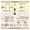
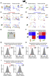
Every day we make decisions critical for adaptation and survival. We repeat actions with known consequences. But we also draw on loosely related events to infer and imagine the outcome of entirely novel choices. These inferential decisions are thought to engage a number of brain regions; however, the underlying neuronal computation remains unknown. Here, we use a multi-day cross-species approach in humans and mice to report the functional anatomy and neuronal computation underlying inferential decisions. We show that during successful inference, the mammalian brain uses a hippocampal prospective code to forecast temporally structured learned associations. Moreover, during resting behavior, coactivation of hippocampal cells in sharp-wave/ripples represent inferred relationships that include reward, thereby "joining-the-dots" between events that have not been observed together but lead to profitable outcomes. Computing mnemonic links in this manner may provide an important mechanism to build a cognitive map that stretches beyond direct experience, thus supporting flexible behavior.
Keywords: cognitive map; cognitive short-cut; hippocampus; humans; inference; memory; mice; prospective code; sharp-wave ripple.
Copyright © 2020 The Author(s). Published by Elsevier Inc. All rights reserved.
Conflict of interest statement
Declaration of Interests The authors declare no competing interests.
Figures
Graphical abstract
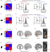
Figure 1
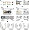
Inference Task Design and Behavioral Performance in Humans and Mice (A) Three-stage inference task. Humans and mice learned to associate auditory cues (Xn) with visual cues (Yn) (“observational learning”); visual cues (Yn) with an outcome (Zn) (“conditioning”), where the outcome was rewarding in set 1 (orange) and neutral in set 2 (green). In the “inference test”, the auditory cues (Xn) were presented in isolation and reward-seeking behavior quantified as a measure of inference from Xn to Zn. (B) Virtual-reality environment used with humans (left), simulating the open-field arena used with mice (right schematic). Outcomes Zn were delivered to a wooden box (humans) or a liquid dispenser (mice). (C and D) Top: timeline for the task in humans (C) and mice (D). Middle: example conditioning trials (schematic). Bottom: example inference test trials (schematic). (C) Middle and bottom: a subset of conditioning trials and all inference test trials were performed inside a 7T scanner. Red square indicates the participant’s response. (D) Middle and bottom: all conditioning and inference test trials were performed within the open-field. Red dotted line delineates outcome area around the dispenser. (E and F) Left of each panel: raw data points for set 1 (orange) and set 2 (green); black dot, mean; black ticks, ±SEM. Right of each panel: behavioral measures of reward-seeking bias shown using bootstrap-coupled estimation (DABEST) plots (Ho et al., 2019). Effect size for the difference between set 1 and 2 (i.e., reward seeking bias), computed from 10,000 bias-corrected bootstrapped resamples (Efron, 2000): black dot, mean; black ticks, 95% confidence interval; filled-curve, sampling-error distribution. (E) Humans exhibited significant reward-seeking bias (percentage of trials where participants wished to visit the wooden box in “set 1” relative to “set 2”) in response to visual cues during conditioning (p < 0.001) and auditory cues during the inference test (p < 0.001). Each data point: average reward-seeking bias of one participant. (F) Mice showed significant reward-seeking bias (percentage of time spent in the outcome area in “set 1” relative to “set 2”) during visual cues in conditioning (p < 0.001; Figures S2A–S2F) and following auditory cues in the inference test (p = 0.005; Figures S2G and S2H). Each data point: average reward-seeking bias of one mouse on a given day. Both humans and mice showed greater reward seeking bias for visual cues Yn (directly paired with Zn), compared to auditory cues Xn (indirectly paired with Zn). See also Figure S1 and Table S4.
Figure S1
In humans and Mice: Inference Task Design and Pre-training Performance, Related to Figure 1 In humans and mice: (A-B) Structure of the inference task in humans and mice. (A) In humans, the experiment was conducted across 3 days. Participants completed observational learning on day 1, conditioning on day 2, and an MRI scan on day 3. During the MRI scan participants were presented with conditioning trials (“reconditioning”) and inference test trials (Figure 1C), presented in a pseudorandom order. (B) In mice, the inference task was conducted across 18 days. Observational learning was conducted across days 1-6, conditioning across days 7-10, and recordings across days 11-18. Each recording day started with a sleep/rest block, after which mice performed conditioning trials (“reconditioning”). The inference test was delivered in 3 separate blocks that were interleaved by reconditioning blocks to minimize extinction effects. At the end of the final inference test, mice were given additional conditioning trials, before being re-exposed to the observational learning. At the end of the recording day mice were recorded during a second sleep/rest block. The two sleep/rest periods were excluded from recording days in mice implanted with optic fibers in the absence of tetrodes. (C) In humans (left) there was a many-to-one mapping between auditory and visual cues. In mice (right) there was a one-to-one mapping between auditory and visual cues. (D) In humans (left) there were four possible visual cues, two in set 1 and two in set 2, which mapped onto two possible outcomes, a monetary reward or a neutral wood-chip. The silver coins or neutral wood-chips could be collected from the wooden box in the corner of the room. In mice (right) there were two possible visual cues, one in set 1 and one in set 2, which mapped onto two possible outcomes, a sucrose (rewarding) or water (neutral) drop delivered to the liquid dispenser. (E-F) Behavioral performance in humans and mice during the pre-training observational learning and conditioning stages of the task (mean ± SEM). (E) In humans. Participants performed the observational learning task until they showed accurate recall of at least 50% of all auditory-visual pairs (left). Participants performed the conditioning task until they reached 100% accuracy on all visual-outcome associations (right). (F) In mice. The observational learning was conducted across 6 days. As expected, mice did not show a reward-seeking bias for cues in set 1 or 2 during this stage of the pretraining (left). Reward-seeking during the observational learning was defined as the percentage time spent in the outcome area in the 20 s period after the auditory cue (Xn) (Figure 1D). After day 3 of the observational learning the time spent in the outcome area following cues in both set 1 and set 2 increased, coinciding with mice being food restricted to 90% their original body weight. The conditioning was conducted across 4 days, during which reward-seeking bias for cues in set 1 compared to set 2 increased (right), indicating that mice learned to associate the visual cues (Yn) with the relevant outcome cues (Zn). Reward-seeking during the conditioning pre-training was defined as the percentage time spent in outcome area during outcome (Zn) availability.
Figure S2
Behavior across All Mice during Conditioning and Inference Test, Related to Figures 1 and 2 In mice: (A-I) Data Analysis with Bootstrap-coupled ESTimation (DABEST) plots (Ho et al., 2019) used to visualize the effect size of behavioral measures of reward seeking bias. Raw data points are shown for set 1 and set 2 in orange and green respectively, with mean ± SEM shown by black-dot and black-ticks respectively. The effect size for the difference between set 1 and 2 (i.e., reward seeking bias) is shown as a sampling-error distribution, computed from 10,000 bias-corrected bootstrapped resamples (Efron, 2000): black-dot, mean; black-ticks, 95% confidence interval; filled-curve, sampling-error distribution; yellow, laser On; gray, laser Off. (A-H) Across recording days in all mice. (A-C) During visual cues (Yn) in conditioning, greater reward-seeking bias was observed for ‘set 1’ relative to ‘set 2’, with reward-seeking bias defined as the percentage time spent in the outcome area (B, p < 0.001), or defined as time spent licking in anticipation of an outcome (C, p < 0.001). Each data point shows the average reward-seeking bias of a single mouse on a given day. (D-F) After visual cues in conditioning, during the outcome period (Zn), greater reward-seeking bias was observed for ‘set 1’ relative to ‘set 2’, with reward-seeking bias defined as the percentage of time spent in the outcome area (E, p < 0.001), or defined as time spent licking the outcome (F, p < 0.001). Each data point shows the average reward-seeking bias of a single mouse on a given day. (G-H) Following auditory cues (Xn) in the inference test, greater reward-seeking bias was observed for ‘set 1’ relative to ‘set 2’, with reward-seeking bias defined as the percentage time spent in the outcome area (p < 0.001; with one data point at coordinates [1,2;0.56,0.35] off the display). (I) In ArchT-GFP mice, dCA1 light delivery during auditory cues (Xn) in the inference test impaired reward-seeking bias observed for ‘set 1’ relative to ‘set 2’ (Figure 2I). This effect was further observed using alternative measures of reward seeking bias shown here, where reward seeking bias is defined as the percentage of trials with visit to outcome area following the auditory cue (laser Off p < 0.001; laser On p = 0.105; laser Off – laser On: t54 = 3.86, p < 0.001).
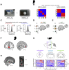
Figure 2
Macroscopic Inference Network in Humans and the Necessary Contribution of dCA1 to Inference in Mice (A) 7T fMRI used to measure the BOLD signal during the inference task (Figure 1C). (B) Significant right hippocampal BOLD signal during correct inference (“correct” – “incorrect” inference: right, t21 = 4.15, p = 0.022; left, t21 = 2.80, p = 0.221; Figure S3A; Table S1). (C) Significant BOLD signal in auditory cortex during inference test trials (“inference trials” – “conditioning trials”: t21 = 14.76, p < 0.001). (D) Psychological-physiological interaction showing differential co-activation with auditory cortex (seed region, C, Figure S3B) on correct versus incorrect inference trials (hippocampus: t21 = 4.23, p = 0.015; and other regions: retrosplenial cortex: t21 = 3.88, p = 0.012; visual cortex: t21 = 4.77, p < 0.001; Table S2). (E–J) In mice. Yellow, laser on; gray, laser off. (E) Schematic: ArchT-GFP viral injections, optic fibers, and tetrodes targeting dCA1 of CamKII-Cre mice for ensemble recording and manipulation. (F) dCA1 (green) ArchT-GFP expression. Scale bar, 500 μm (left), 50 μm (right). (G) Raster plot showing photo-silencing of spiking activity for an example dCA1 pyramidal cell from an ArchT-GFP mouse. (H) Light-induced changes in firing rate for simultaneously recorded dCA1 pyramidal cells in an example ArchT-GFP mouse (laser on: t30 = −10.86, p < 0.001; laser off – laser on: t30 = 10.88, p < 0.001). Rate changes expressed for each cell as the differences between laser on and laser off firing over the sum (scores; center line, median; box limits, upper and lower quartiles; whiskers, 1.0× interquartile range). (I and J) Left panel: schematic of light delivery. Bottom right panel: raw data points for set 1 (orange) and set 2 (green); black dot, mean; black ticks, ± SEM. Top right panel: behavioral measures of reward seeking bias shown using DABEST plots, as in Figures 1E and 1F. (I) dCA1 light delivery during auditory cues Xn in the inference test impaired reward-seeking bias in ArchT-GFP mice (set 1 – set 2: laser off p < 0.001; laser on p = 0.794; laser off – laser on: t54 = 2.25, p = 0.029; alpha set to 0.05; Figure S2I) but not in GFP control mice (set 1 – set 2: laser off p < 0.001; laser on p < 0.001; laser off – laser on: t46 = −0.85, p = 0.399; alpha set to 0.05). The significant reward-seeking biases (ArchT-GFP laser off; GFP control laser off and on) remained significant with Bonferroni correction for four comparisons, alpha set to 0.013. A significant interaction was also observed between the ArchT-GFP and GFP control mice (group × laser interaction, two-way ANOVA, F1,100 = 4.42, p = 0.038). (J) dCA1 optogenetic silencing during visual cues Yn, presented after the inference task was complete, did not impair reward-seeking bias in ArchT-GFP mice (set 1 – set 2: laser off p = 0.003; laser on p < 0.001; laser off – laser on: t26 = −0.14, p = 0.891). See also Table S4.
Figure S3
Regions of Interest and RSA during the Inference Test in Humans, Related to Figures 2 and 4 In humans: (A) An anatomical ROI in the hippocampus. This ROI was used to correct for multiple comparisons across the hippocampal volume (Figure 2B). (B) An ROI in auditory cortex was defined from a contrast comparing BOLD signal during inference test trials to conditioning trials (Figure 2C). This ROI was then used as a seed region for a Psychological-Physiological Interaction analysis which identified brain regions that differentially co-activate with auditory cortex across correct and incorrect trials in the inference test (Figure 2D). (C) During correctly inferred trials in the inference test, searchlight RSA was applied to fMRI data in humans to identify brain regions showing representational similarity between auditory cues Xn and visual cues Yn. A model representational similarity matrix (Figure 4E) that mapped the auditory-to-visual associations learned during the inference task was compared with the activity patterns across voxels extracted from each searchlight, using a summary statistic estimated as follows: [average within association XnYn correlations from RSM main diagonal] – [average between association XnYm correlations from RSM off-diagonals]. (D) The searchlight analysis described in (C) revealed significant auditory-visual mappings in the hippocampus (t21 = 4.76, p = 0.025; peak-level FWE corrected using small-volume correction method), as observed in Figure 4. (E) The searchlight analysis described in (C) further revealed significant auditory-visual mappings in the visual cortex (t21 = 4.94, p = 0.012, FWE whole-brain corrected at the cluster-level). T-statistic maps are thresholded at p < 0.01 uncorrected for visualization purposes only. (F) In humans, RSA was applied to BOLD signal extracted from a region of interest (ROI) in the hippocampus, defined from the univariate contrast reported in Figure 2B, thresholded at p < 0.01 uncorrected. (G) Applying RSA to hippocampal activity we modeled the mappings from Xn in the inference test to Yn in conditioning, both independent of the value of the associated Zn (left), and dependent upon the value of the associated Zn (right). We then used multiple regression to regress the data onto these two models, to assess evidence for prospective representation of visual cues Yn over and above representation of the value associated with the visual cues. (H) Using multiple regression described in G, during correct inference, activity patterns in the hippocampus significantly predicted mappings from Xn to Yn, independent of the value of the associated Zn cues (correct and incorrect inference: Z21 = 2.01, p = 0.022 and Z21 = −1.07, p = 0.858; mean ± SEM). The group mean was further compared against a null distribution generated by permuting the identity labels assigned to the auditory cues Xn (correct and incorrect inference: p = 0.006 and p = 0.854). (I) Using multiple regression described in G, during correct inference, activity patterns in the hippocampus did not significantly predict mappings from Xn to Yn, dependent upon the value of the associated Zn cues (correct and incorrect inference: Z21 = −0.39, p = 0.652 and Z21 = 1.23, p = 0.109; mean ± SEM). The group mean was further compared against a null distribution generated by permuting the identity labels assigned to the auditory cues Xn (correct and incorrect inference: p = 0.839 and p = 0.070). Thus, during inferential choice hippocampal activity in humans prospectively represents visual cues Yn over and above representation of the value of the associated Zn cues.
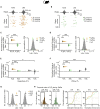
Figure 3
dCA1 Neuronal Representation of Inference Task Cues in Mice (A) Top and middle rows: Raster plots and peri-stimulus time histograms for 6 example neurons, each showing firing response to one of the 6 task cues (Xn, Yn, and Zn) (Figure 1A). Bottom row: heatmap showing the average Z scored firing rate (Hz) of 60 example neurons in response to task cues, ordered according to the preferred cue on the y axis. (B) For each recorded neuron, the average Z scored firing rate across each trial was filtered by the “decision point” (Figure S4) and regressed onto a GLM that modeled all task cues and the mouse’s average speed. GLM for an example neuron is shown. (C) For each cue, the regression weights from all neuron-specific GLMs are shown for an example recording day. Neurons with regression weights more than 2 SD from the group mean were assigned to a cue-specific ensemble and color-coded for visualization (orange, set 1; green, set 2). (D) UpSet plot (Lex et al., 2014) showing the number of neurons within and shared across each cue-specific ensemble. Only a minority of neurons contributed to more than one cue-specific ensemble. (E and F) Average Z scored firing rate of neurons in the Xn,Yn, and Zn ensembles in response to each task cue. (E) For an example recording day, the average response of each neuron allocated to a cue-specific ensemble is shown. (F) Across all recording days, the average response of all neurons in a given cue-specific ensemble is shown (mean ± SEM). See also Table S4.
Figure 4
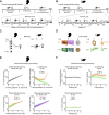
Hippocampal Prospective Memory Code during Correct Inference in Humans and Mice (A and B) During auditory cues Xn in the inference test, the BOLD signal (humans; A) and the Z scored firing rate of each dCA1 neuron (mice; B) were regressed onto the behavioral performance (correct versus incorrect inference) using a GLM. During Xn, the extracted regression weights (mean ± SEM) were significantly positive for correct versus incorrect inference (humans: t21 = 4.04, p < 0.001; mice: t99 = 10.24, p < 0.001). (C and D) In humans (C) and mice (D) hippocampal activity patterns during auditory cues in the inference test and during visual cues in conditioning were compared using RSA to establish a cross-stimulus representational similarity matrix (RSM). In mice, data were filtered by the “decision point” on each trial. (E and F) Average RSMs in humans (E) and mice (F), for the model (predicted results) and the data (observed results), split by behavioral performance in the inference test. Rank-transformed and scaled between (0 to 1) for visualization. (G and H) In both humans (G) and mice (H), hippocampal activity during correctly inferred auditory cues Xn in the inference test significantly predicted the associated visual cue Yn, ([average within association XnYn correlations, RSM main diagonal] – [average between association XnYm correlations, RSM off-diagonals]; correct and incorrect inference; humans: Z21 = 2.24, p = 0.013 and Z21 = 0.71, p = 0.238; mice: Z17 = 3.00, p = 0.001 and Z17 = 0.39, p = 0.348; mean ± SEM). In both species, the group mean was compared against a null distribution generated by permuting the identity labels of cues Xn (correct and incorrect inference; humans: p = 0.005 and p = 0.620; mice: p < 0.001 and p = 0.417; alpha set to 0.05). All statistical tests for correctly inferred trials remained significant with Bonferroni correction to account for two comparisons (correctly and incorrectly inferred), alpha set to 0.025. See also Figures S3 and S4 and Table S4.
Figure S4
In Mouse dCA1, Representational Similarity between Activity Patterns for Xn and Yn in Set 1 Is Not Explained by Spatial Trajectory, Related to Figures 3, 4, 5, and 6 In mice: (A-D) Overlaid trajectory for an example mouse during visual cues (Yn) and auditory cues (Xn). Blue indicates the start of the trajectory and red indicates the end of the trajectory. Left hand panels: complete trajectories during the cue. Right hand panels: trajectories filtered by the “decision point” of the mouse, as applied in Figures 3, 4, 5, and 6. The “decision point” of the mouse is defined as the time point where the speed of the mouse was below 5cm/s prior to visiting the outcome area on that trial (see STAR Methods). Filtering the trial data by the decision point eliminated time periods where the mouse was at or near the dispenser, thus controlling for spatial confounds in set 1. (A) Trajectories during visual cue Y1 from set 1. (B) Trajectories during visual cue Y2 from set 2. (C) Trajectories during auditory cues Xn from set 1 and 2 for correctly inferred trials. (D) Trajectories during auditory cues Xn from set 1 and 2 for incorrectly inferred trials. (E) Schematic showing birds-eye view of the open field used for the example mouse shown in A-D. (F) The average representational similarity matrices (RSMs) across recording days for spatial trajectories during cues Xn and Yn, after filtering by the decision point and dividing the data by performance in the inference test. Rank-transformed and scaled between [0 to 1] for visualization purposes. (G-H) The average representational similarity for ‘within set’ versus ‘between set’ spatial trajectories across cues Xn and Yn, after filtering by the decision point and splitting by performance in the inference test. The group mean was compared against a null distribution generated by permuting the identity labels assigned to the auditory cues Xn. (G) Across both set 1 and 2, spatial trajectories during the auditory cues Xn significantly predicted the trajectories for the associated visual cue Yn, ([within set XnYn correlation] – [between set XnYn correlation], ‘correct inference’ p = 0.014, ‘incorrect inference’ p = 0.687). (H) Across set 1 alone, spatial trajectories during the auditory cues Xn did not significantly predict the trajectories for the associated visual cue Yn, ([within XnYn correlation] – [between XnYn correlation], ‘correct inference’ p = 0.957, ‘incorrect inference’ p = 0.151). (I) Across set 1 alone, the single-unit activity in neurons recorded from dCA1 during auditory cues Xn significantly predicted the activity patterns for the associated visual cue Yn during correct but not incorrect inference ([within set XnYn correlation] – [between set XnYn correlation]). The group mean was compared against a null distribution generated by permuting the identity labels assigned to the auditory cues Xn (‘correct inference’ p = 0.002, ‘incorrect inference’ p = 0.865). Given the absence of significant spatial correlations for set 1 shown in H, this result shows that during correct inference, dCA1 ensemble activity predicted the associated cue Yn over and above the spatial location of the animal.
Figure 5
dCA1 Neuronal Spike Timing Supports a Prospective Code during Inference in Mice (A and B) During inference, we assessed the spike time relationships between neuronal ensembles representing cues Xn and Yn (Figures 3C and 3D). The cross-correlogram for spike counts in each pair of XnYn cells showed the spiking probability of neuron Yn relative to neuron Xn. Shown: example cell pair for set 1 (A) and set 2 (B) where neuronal ensembles representing cues Xn and Yn fire sequentially, preserving the learned temporal dynamics of task cues. Right panel: change in joint probability of XnYn spiking relative to baseline (average joint probability 50 ms prior to Xn spikes). (C and D) During cues Xn in the inference test we estimated the Z scored spike-triggered average for neurons in ensembles Yn (shown in C) or Ym (shown in D), within a 200-ms window relative to spikes in neurons representing Xn. DABEST plots used to compare the difference in the mean Z scored spike-triggered average for both Yn and Ym, “after” minus “before” spikes in Xn: black dot, mean; black ticks, 95% confidence interval; filled-curve, sampling-error distribution. Yn, but not Ym, neurons typically fired after Xn neurons (“after” – “before” Xn spike discharge: red within-set neuronal pairs shown in C, X1Y1 and X2Y2, p < 0.001; gray cross-set neuronal pairs shown in D, X1Y2 and X2Y1, p = 0.983; Figure S5). Thus, despite the absence of Yn cues, spiking across XnYn cell pairs preserved the learned temporal statistics from the observational learning stage. See also Figure S4 and Table S4.
Figure S5
Spike Time Relationships between dCA1 Neurons during Inference, Related to Figure 5 In mice: (A-B) During the auditory cues Xn in the inference test we estimated the Z-scored spike-triggered average for neurons in ensembles Xn, within a 200-ms window relative to the spike times of neurons in ensembles Yn. For each cell pair we assessed the difference in the mean Z-scored spike-triggered average for Xn during the 100-ms interval “after” minus “before” spikes in Yn. The effect size for the difference (“after” – “before”, right-hand panel) was estimated by computing 10,000 bias-corrected bootstrapped resamples (Efron, 2000) and visualized using DABEST plots (Ho et al., 2019): black-dot, mean; black-ticks, 95% confidence interval; filled-curve, sampling-error distribution; red, within-set cell pairs; gray, cross-set cell pairs. (A) For all within-set neuronal pairs (X1Y1 and X2Y2), the Z-scored spike-triggered average for Xn was significantly higher during the 100 ms before Yn spike discharge (“after” – “before” Yn neuron spike: p < 0.001), showing that during presentation of the auditory cues Xn in the inference test, Xn neurons tend to spike before Yn neurons, thus preserving the temporal statistics of cue presentation from the observational learning stage of the task (Figure 1A). (D) For all cross-set neuronal pairs (X1Y2 and X2Y1), there was no significant temporal bias in the Z-scored spike-triggered average for Xm when comparing the 100 ms “after” minus “before” spikes in Yn (“after” – “before” Xn neuron spike: p = 0.640).
Figure 6
Inferred Outcomes Are Represented in mPFC and Midbrain (A–D) In humans (A and B) and mice (C and D) hippocampal activity patterns during auditory cues Xn in the inference test were compared with activity patterns during outcome Zn in conditioning using RSA. In mice, time bins with SWRs were excluded. Activity patterns during Xn in the inference test, but not Zn in conditioning, were filtered by the “decision point” on each trial, such that representations of Zn were spatially decoupled from representations of Yn. Hippocampal activity in humans and mice did not significantly predict activity associated with the relevant outcome Zn ([average within association XnZn correlations, RSM main diagonal] – [average between association XnZm correlations, RSM off-diagonals]; correct and incorrect inference; humans, conditional on intermediary cues: Z21 = −0.06, p = 0.526, and Z21 = −0.75, p = 0.772; mice: Z17 = −0.87, p = 0.808; and Z17 = 0.44, p = 0.331; mean ± SEM), including when comparing the group mean against a null distribution generated by permuting the identity labels for cues Xn (correct and incorrect inference; humans: p = 0.464, and p = 0.868; mice: p = 0.829 and p = 0.176). See Figure S6C for results in humans unconditional on intermediary cues. By contrast, robust dCA1 representation of Zn was observed in mice during experience of outcome Zn in conditioning trials (Figure 3). (E–J) In humans, searchlight RSA with multiple regression (Figures S6D and S6E) was used to identify regions showing representational similarity between auditory cues Xn in the inference test and outcomes Zn in conditioning. During correctly inferred cues Xn, both the mPFC (F) and putative dopaminergic midbrain (G) regions showed significant representation of the associated Zn, conditional on sensory cues that predicted the outcome as shown in the model RSM in (E) (F, mPFC: t21 = 5.09, p = 0.003; G, midbrain: t21 = 5.56, p < 0.001; thresholded at p < 0.01 uncorrected for visualization purposes only). This result held for cues in set 2 as shown in the model RSM in (H) (I: mPFC: t21 = 4.60, p = 0.006; J, midbrain: t21 = 3.37, p = 0.027; peak-level FWE corrected using small-volume correction; Figures S6F and S6G; thresholded at p < 0.01 uncorrected for visualization purposes only). See also Figure S4 and Tables S3 and S4.
Figure S6
Representation of the Inferred Outcome in Humans and Triple-Site Recording of Neuronal Ensembles in dCA1, mPFC, and VTA in Mice, Related to Figure 6 (A-G) In humans. (A) RSA was assessed between auditory cues Xn during the inference test, and outcome cues Zn during the conditioning trials. (B) Using multiple regression, representational similarity between the auditory cues Xn and outcome cues Zn was assessed using two models. The first model (left) mapped the relationship between the auditory cues Xn and the associated outcomes Zn, conditional on the intermediary visual cues Yn (Figures 6A and 6B). The second model (right) mapped relationships between the auditory cues Xn and the associated outcomes Zn, unconditional on the intermediary visual cues Yn. (C) RSA was applied to the BOLD signal extracted from the hippocampal ROI shown in Figure S3F. Using multiple regression to regress the data onto the two models described in B, during the inference test we assessed evidence for representation of outcome cues Zn in the hippocampus. During both correctly inferred and incorrectly inferred trials in the inference test, hippocampal activity did not significantly predict activity associated with the relevant outcome cues Zn, unconditional on intermediary visual cues Yn (correct and incorrect inference: Z21 = 0.91, p = 0.182 and Z21 = 0.84, p = 0.199). The group mean was further compared against a null distribution generated by permuting the identity labels assigned to the auditory cues Xn (correct and incorrect inference: p = 0.199 and p = 0.289). Results conditional on the intermediary visual cues Yn are shown in Figures 6A and 6B. (D-E) Searchlight RSA in humans was used to identify brain regions showing representational similarity between auditory cues Xn and outcomes Zn for cues in both set 1 and 2 (D) and for cues in set 2 only (E), where Z2 represents a neutral cue. (F-G) ROIs used to correct for multiple comparisons within the medial prefrontal cortex and VTA (Figures 6I and 6J). (F) An ROI in the medial prefrontal cortex, defined from functional map showing evidence for novel conjunctive representations in medial prefrontal cortex (Barron et al., 2013). (G) An ROI in the VTA, defined from a functional map identifying midbrain activation to reward-prediction error (Klein-Flügge et al., 2011). (H) In mice. Upper: Schematic showing the 3 simultaneously recorded brain regions: medial prefrontal cortex (mPFC), hippocampal dCA1 and ventral tegmental area (VTA) (n = 4 mice). Lower: Heatmap showing spiking activity of 3x30 example neurons recorded across the mPFC, dCA1 and VTA. For each heatmap, each row shows the Z-scored firing rate (Hz) of a given neuron within 100 ms bins, averaged across multiple trials in which sucrose is delivered to the outcome dispenser within the open field shown in Figure 1B. For each brain region the y axis is organized to first show those neurons that show an increase in their spiking activity in response to sucrose delivery. This triple-site recording shows that spiking activity in these three brain regions can be modulated in relation to experience of reward, and also illustrates how triple-site recordings may be used in the future to investigate findings reported in humans at a cellular level (Figure 6).
Figure 7
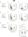
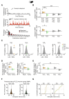
Hippocampal Spiking Represents Inferred Relationships during SWRs (A and B) In mice. Top: mean ripple-band (135–250 Hz) dCA1 oscillations during awake rest in the inference task. Bottom: co-firing of example X1Y1Z1 (A) and X2Y2Z2 (B) neuronal triplets across SWRs during early and late recording days. (C–G) From early to late days (recording days 1–4 versus 5–8; Figure S1B), we estimated the normalized probability of SWRs co-representing neuronal triplets/doublets during awake rest in the inference test. The effect size for the difference between early and late days is shown using a DABEST plot: black dot, mean; black ticks, 95% confidence interval; filled-curve, sampling-error distribution. Tukey’s post hoc multiple comparison test was used to assess the difference in group means following ANOVA. (C) From early to late days, we observed a significant interaction in the probability of SWRs representing set 1 (X1Y1Z1) versus set 2 (X2Y2Z2) neuronal triplets (set × day interaction, two-way ANOVA: F(1,1573) = 28.14, p < 0.001). Tukey’s post hoc test showed a significant increase in SWRs representing set 1 (X1Y1Z1) triplets (p < 0.001). Compared to a null distribution generated by permuting the identity labels of ensemble neurons (Figures 3C and 3D), we again observed a significant increase in SWRs representing set 1 (X1Y1Z1) triplets (p = 0.002). (D) From early to late days we observed a significant interaction in the probability of SWRs representing X1Y2Z1 versus X2Y1Z2 triplets, where the identity of Ym cells were from the opposite set (set × day interaction, two-way ANOVA: F(1,900) = 33.97, p < 0.001). Tukey’s post hoc test showed a significant increase in SWRs representing X1Y2Z1 triplets (p < 0.001). Compared to a null distribution generated by permuting the identity labels of ensemble neurons (Figures 3C and 3D), we again observed a significant increase in SWRs representing X1Y2Z1 (p = 0.014). (E and F) From early to late days we observed a significant interaction in the probability of SWRs representing neuronal pairs for the inferred relationship in set 1 (X1Z1) versus set 2 (X2Z2), both regardless of Yn neurons (E) and in the absence of Yn neurons (F) (set × day interaction, two-way ANOVA: E, F(1,285) = 24.04, p < 0.001; F, F(1,1716) = 45.8, p < 0.001). Tukey’s post hoc test showed a significant increase in SWRs representing set 1 (X1Z1) pairs (E, p < 0.001; F, p < 0.001). This result was not explained by a mere increase in SWRs representing Z1 as the interaction remained significant when comparing SWRs representing set 1 (X1Z1) versus cross-set (X2Z1) pairs (set × day interaction, two-way ANOVA: E, F(1,260) = 5.14, p = 0.024; F, F(1,1642) = 18.08, p < 0.001). (G) To further control for a mere increase in SWRs representing Z1 cues in (F), we compared the group mean against a null distribution generated by permuting the SWRs with Xn spikes, while holding Zn spikes fixed. From early to late days the probability of SWRs showing coactivity between neurons representing X1 and Z1, but not X2 and Z1, increased relative to the respective null distribution (X1Z1: p < 0.001; X2Z1: p = 0.193; Figure S7C). (H) Inter-spike intervals for Xn and Zn neuron pairs. Across all neuron pairs, the percentage of pairs where Z1 fired before X1 was significant (p < 0.001, binomial test with alpha set to 0.05). The percentage of pairs where Z2 fired before X2 did not differ from 50% (p = 0.101, Binomial test with alpha set to 0.05). Set 1 in orange; set 2 in green. The effect for set 1 remained significant with Bonferroni correction for two comparisons (set 1 and set 2) and alpha at 0.025. See also Table S4.
Figure S7
During SWRs, Hippocampal Co-firing Autocompletes Inferred Relationships, Related to Figure 7 In mice: (A) Upper: Example instantaneous speed (cm/s) during a rest/sleep session of a recording day (Figure S1B) when the mouse was in the “sleep box”. Middle: Example instantaneous speed (cm/s) during an inference test session (Figure S1B) when the mouse was in the open field (Figure 1B). Notably, the mouse is more active during the inference test relative to the rest/sleep session shown in A. Lower: The distribution of instantaneous speed (mean ± SEM) recorded across all mice during rest sessions and during the inference task. The proportion of time spent immobile (0-1cm/s) was greater during rest sessions, while the proportion of time spent active (> 1cm/s) was greater during the inference task. (B) To further measure firing associations between hippocampal neurons during SWRs (Figure 7), we used a second approach reported previously (Dupret et al., 2010; McNamara et al., 2014). In brief, this co-firing measure involved first calculating for each cell the instantaneous firing rate counts within each SWR of a given recording session, before computing the Pearson correlation coefficient between the instantaneous firing rate counts for each cell pair, across all SWRs of that recording session. Between early and late recording days, we then tested the difference in pairwise co-firing for cue-defined cell pairs against zero and estimated DABEST plots as described in Figures 1E and 1F. Tukey’s post hoc multiple comparison test was used to further assess the difference in group means following ANOVA. Upper: From early to late recording days we observed a significant interaction in SWR co-firing for set 1 versus set 2 cell pairs (set x day interaction, two-way ANOVA: F(1,2005) = 13.68, p < 0.001). Tukey’s post hoc test revealed a significant increase in SWR co-firing for set 1 cell pairs ([X1Y1, Y1Z1, X1Z1]: p = 0.040) and a significant decrease in set 2 cell pairs ([X2Y2, Y2Z2, X2Z2]: p = 0.040). This result was not explained by a mere increase in the probability of SWRs representing Z1: the interaction remained significant when comparing the SWR co-firing for set 1 and equivalent across-set ([X2Y1, Y2Z1, X2Z1]) cell pairs (two-way ANOVA: F(1,1965) = 13.93, p < 0.001), where Tukey’s post hoc test also revealed a significant increase in SWR co-firing for set 1 cell pairs ([X1Y1, Y1Z1, X1Z1]: p = 0.015). Lower: From early to late recording days we observed a significant interaction in SWR co-firing for set 1 versus set 2 cell pairs representing the inferred (but not directly observed) relationship (set 1: [X1Z1]; set 2: [X2Z2]; set x day interaction, two-way ANOVA: F(1,365) = 6.45, p = 0.012). However, Tukey’s post hoc test did not reveal a significant increase in SWR co-firing for set 1 cell pairs ([X1Z1]: p = 0.235). Critically, unlike the analyses presented in Figure 7, the methodological approach implemented here did not control for SWR co-firing of cells representing the intermediary visual cues Yn. (C) From early to late recording days we observed a significant increase in the probability of SWRs representing neuronal pairs for the inferred relationship in set 1 (X1Z1) in the absence of Yn neurons (Figure 7F). To control for a mere change in SWRs representing task cues from early to late recording days, we compared the group mean for both within-set (X1Z1 and X2Z2) and cross-set (X1Z2 and X2Z1) neuronal pairs against a null distribution generated by permuting the SWRs in which Xn neuronal spikes occurred in each pair, while holding the relevant Zn neuronal spikes fixed and thus preserving the average firing rate of both Xn and Zn cells. This analysis revealed a significant increase in probability of SWRs representing the inferred relationship from set 1 (X1Z1, p < 0.001), but no significant change in the probability of SWRs representing all other neuronal pairs (X2Z2, p = 0.281; X1Z2, p = 0.934; X2Z1, p = 0.193). See also Figure 7G. (D-E) From early to late recording days, the normalized probability of SWRs co-representing neuronal triplets during periods of rest/sleep sessions recorded in the “sleep box” at the beginning and end of the recording day (Figure S1B). The effect size for the difference between early and late is shown using DABEST plots as described in Figures 1E and 1F. Tukey’s post hoc multiple comparison test was used to further assess the difference in group means following ANOVA. (D) From early to late recording days we observed a significant interaction in SWRs representing set 1 (X1Y1Z1) versus set 2 (X2Y2Z2) neuronal triplets (set x day interaction, two-way ANOVA: F(1,1106) = 15.86, p < 0.001). Tukey’s post hoc test revealed a significant increase in the probability of SWRs representing set 1 (X1Y1Z1) neuronal triplets (p < 0.001). From early to late recording days there was no significant interaction in the probability of SWRs representing set 1 (X1Y2Z1) versus set 2 (X2Y1Z2) neuronal triplets, where the identify of Yn cells were from the opposite set (set x day interaction, two-way ANOVA: F(1,828) = 2.67, p = 0.102). However, Tukey’s post hoc test revealed a significant increase in the probability of SWRs representing set 1 (X1Y2Z1) neuronal triplets (p = 0.024). (E) From early to late recording days there was no significant interaction in the probability of SWRs representing neuronal pairs for the inferred relationship in set 1 (X1Z1) versus set 2 (X2Z2), regardless of Yn neurons (set x day interaction, two-way ANOVA: F(1,224) = 1.41, p = 0.237). However, Tukey’s post hoc test revealed a significant increase in SWRs representing set 1 (X1Z1) neuronal pairs (p = 0.005). This result was not explained by a mere increase in SWRs representing Z1 as a significant interaction was observed when comparing SWRs representing set 1 (X1Z1) versus across-set (X2Z1) neuronal pairs (set x day interaction, two-way ANOVA: F(1,187) = 10.94, p = 0.001). Overall, during offline periods of rest/sleep the increase in SWRs co-representing X1Z1 neuronal pairs showed less specificity than that observed for SWRs recorded in periods of quiet wakefulness during the inference test (Figures 7C–7F). (F-G) Inter-spike intervals for Xn and Zn neuron pairs (see STAR Methods). Unlike SWRs recorded during awake rest in the inference test (Figure 7H), during periods of sleep/rest in the “sleep box” the number of neuron pairs where Z1 fired before X1 was not significant (p = 0.195, Binomial test). Similarly, the number of neuron pairs where Z2 fired before X2 did not differ from 50% (p = 0.519, Binomial test). Set 1 in orange; set 2 in green.
Similar articles
- A Unified Dynamic Model for Learning, Replay, and Sharp-Wave/Ripples.
Jahnke S, Timme M, Memmesheimer RM. Jahnke S, et al. J Neurosci. 2015 Dec 9;35(49):16236-58. doi: 10.1523/JNEUROSCI.3977-14.2015. J Neurosci. 2015. PMID: 26658873 Free PMC article. - Dorsal and Ventral Hippocampal Sharp-Wave Ripples Activate Distinct Nucleus Accumbens Networks.
Sosa M, Joo HR, Frank LM. Sosa M, et al. Neuron. 2020 Feb 19;105(4):725-741.e8. doi: 10.1016/j.neuron.2019.11.022. Epub 2019 Dec 18. Neuron. 2020. PMID: 31864947 Free PMC article. - Coordinated Interaction between Hippocampal Sharp-Wave Ripples and Anterior Cingulate Unit Activity.
Wang DV, Ikemoto S. Wang DV, et al. J Neurosci. 2016 Oct 12;36(41):10663-10672. doi: 10.1523/JNEUROSCI.1042-16.2016. J Neurosci. 2016. PMID: 27733616 Free PMC article. - Hippocampal ripples as a mode of communication with cortical and subcortical areas.
Todorova R, Zugaro M. Todorova R, et al. Hippocampus. 2020 Jan;30(1):39-49. doi: 10.1002/hipo.22997. Epub 2018 Nov 13. Hippocampus. 2020. PMID: 30069976 Review. - Non-structured spike sequences of hippocampal neuronal ensembles in awake animals.
Sasaki T. Sasaki T. Neurosci Res. 2019 May;142:1-6. doi: 10.1016/j.neures.2018.05.005. Epub 2018 May 26. Neurosci Res. 2019. PMID: 29842894 Review.
Cited by
- Hippocampal sequences span experience relative to rewards.
Sosa M, Plitt MH, Giocomo LM. Sosa M, et al. bioRxiv [Preprint]. 2024 Feb 4:2023.12.27.573490. doi: 10.1101/2023.12.27.573490. bioRxiv. 2024. PMID: 38234842 Free PMC article. Preprint. - Concepts as plug & play devices.
Shea N. Shea N. Philos Trans R Soc Lond B Biol Sci. 2023 Feb 13;378(1870):20210353. doi: 10.1098/rstb.2021.0353. Epub 2022 Dec 26. Philos Trans R Soc Lond B Biol Sci. 2023. PMID: 36571131 Free PMC article. - Theta oscillations coordinate grid-like representations between ventromedial prefrontal and entorhinal cortex.
Chen D, Kunz L, Lv P, Zhang H, Zhou W, Liang S, Axmacher N, Wang L. Chen D, et al. Sci Adv. 2021 Oct 29;7(44):eabj0200. doi: 10.1126/sciadv.abj0200. Epub 2021 Oct 27. Sci Adv. 2021. PMID: 34705507 Free PMC article. - Coordinating brain-distributed network activities in memory resistant to extinction.
Clarke-Williams CJ, Lopes-Dos-Santos V, Lefèvre L, Brizee D, Causse AA, Rothaermel R, Hartwich K, Perestenko PV, Toth R, McNamara CG, Sharott A, Dupret D. Clarke-Williams CJ, et al. Cell. 2024 Jan 18;187(2):409-427.e19. doi: 10.1016/j.cell.2023.12.018. Cell. 2024. PMID: 38242086 Free PMC article. - Anterior cingulate neurons signal neutral cue pairings during sensory preconditioning.
Hart EE, Gardner MPH, Schoenbaum G. Hart EE, et al. Curr Biol. 2022 Feb 7;32(3):725-732.e3. doi: 10.1016/j.cub.2021.12.007. Epub 2021 Dec 21. Curr Biol. 2022. PMID: 34936884 Free PMC article.
References
- Battaglia F.P., Benchenane K., Sirota A., Pennartz C.M.A., Wiener S.I. The hippocampus: hub of brain network communication for memory. Trends Cogn. Sci. 2011;15:310–318. - PubMed
- Brogden W.J. Sensory pre-conditioning. J. Exp. Psychol. 1939;25:323–332. - PubMed
- Buckner R.L. The role of the hippocampus in prediction and imagination. Annu. Rev. Psychol. 2010;61:27–48. - PubMed
- Bunsey M., Eichenbaum H. Conservation of hippocampal memory function in rats and humans. Nature. 1996;379:255–257. - PubMed
Publication types
MeSH terms
Grants and funding
- MC_UU_12024/3/MRC_/Medical Research Council/United Kingdom
- BB/N0059TX/1/BB_/Biotechnology and Biological Sciences Research Council/United Kingdom
- 203964/WT_/Wellcome Trust/United Kingdom
- 104765/WT_/Wellcome Trust/United Kingdom
- MC_UU_00003/4/MRC_/Medical Research Council/United Kingdom
- 203139/WT_/Wellcome Trust/United Kingdom
- MR/T031344/1/MRC_/Medical Research Council/United Kingdom
- 203836/WT_/Wellcome Trust/United Kingdom
LinkOut - more resources
Full Text Sources
Other Literature Sources
Molecular Biology Databases
