Coupled social and ecological change drove the historical extinction of the California grizzly bear (Ursus arctos californicus)

Alexis M Mychajliw et al. Proc Biol Sci. 2024.

Abstract

Large carnivores (order Carnivora) are among the world's most threatened mammals due to a confluence of ecological and social forces that have unfolded over centuries. Combining specimens from natural history collections with documents from archival records, we reconstructed the factors surrounding the extinction of the California grizzly bear (Ursus arctos californicus), a once-abundant brown bear subspecies last seen in 1924. Historical documents portrayed California grizzlies as massive hypercarnivores that endangered public safety. Yet, morphological measurements on skulls and teeth generate smaller body size estimates in alignment with extant North American grizzly populations (approx. 200 kg). Stable isotope analysis (_δ_13C, _δ_15N) of pelts and bones (n = 57) revealed that grizzlies derived less than 10% of their nutrition from terrestrial animal sources and were therefore largely herbivorous for millennia prior to the first European arrival in this region in 1542. Later colonial land uses, beginning in 1769 with the Mission era, led grizzlies to moderately increase animal protein consumption (up to 26% of diet), but grizzlies still consumed far less livestock than otherwise claimed by contemporary accounts. We show how human activities can provoke short-term behavioural shifts, such as heightened levels of carnivory, that in turn can lead to exaggerated predation narratives and incentivize persecution, triggering rapid loss of an otherwise widespread and ecologically flexible animal.

Keywords: California; carnivore; extinction; historical ecology; human–wildlife conflict; stable isotope.

PubMed Disclaimer

Conflict of interest statement

We declare we have no competing interests.

Figures

Figure 1.

Geographical distribution of California grizzly bear (Ursus arctos californicus) specimens used in this study. (a) Specimens represent pre- (n = 17) and post- (n = 40) 1542 time bins (time of European colonization) and are grouped into North/Inland, Central Coast (including detailed inset maps) and South Coast regions. Spatial patterns in stable isotope values of (b) nitrogen (_δ_15N) and (c) carbon (_δ_13C), with inset map featuring a portion of the Central Coast in all panels. Symbols courtesy of Phylopic (

http://phylopic.org

Figure 2.

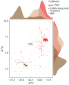
(a) Biplot showing stable isotope values (_δ_15N, _δ_13C) for California grizzlies and their potential food items (mean ± s.d.) statewide across the pre and post periods, not including trophic discrimination factor but with all relevant tissue and Suess corrections. Note that the same plant value was used across periods (see also electronic supplementary material, figure S7). A = anadromous fish, F = freshwater fish. (b) Biplot showing the individual grizzlies in the pre (grey) and post (red) 1542 periods, as well as their means ± 1 s.d. (produced using the R package tRophicPosition [36]. Also shown in the margins are the distributions of _δ_15N (right) and _δ_13C (top) values for these two. groups. Symbols courtesy of Phylopic (

http://phylopic.org

Figure 4.

(a) Stable isotope values of Monarch's hair (purple square) and bone (purple circle) compared with average hair (black square) and bone (black circle) values (mean ± 1 s.d.) and individual data (grey dots) obtained from grizzlies from California's South Coast post-1542. (b) Monarch, in captivity at the San Francisco Woodward Gardens Zoo, C. Hart Merriam Pictorial Collection (Bancroft Library). (c) Kernel estimates and histograms showing the frequency distributions of the body mass (kilogram) of California grizzlies estimated using morphologically based regression equations and reports in historical newspapers and archives from [12]. At the top of c are images of Monarch's skeleton (left) and an advertisement for a California grizzly exhibit (right, Bancroft Library).

Figure 3.

Biplot of stable isotope values for individual livestock (tan), deer (brown) and grizzlies (red) in the post-1542 period, as well as their means ± 1 s.d. (produced using the R package tRophicPosition [36]. Also shown in the margins are the distributions of _δ_15N (right) and _δ_13C (top) values for these three groups. All plots account for Suess corrections. Symbols courtesy of Phylopic (

http://phylopic.org

References

1. Akçakaya HR, et al. 2018. Quantifying species recovery and conservation success to develop an IUCN Green List of Species. Conserv. Biol. 32, 1128-1138. (10.1111/cobi.13112) - DOI - PubMed
1. Grace MK, et al. 2021. Testing a global standard for quantifying species recovery and assessing conservation impact. Conserv. Biol. 35, 1833-1849. (10.1111/cobi.13756) - DOI - PubMed
1. Chapron G, et al. 2014. Recovery of large carnivores in Europe's modern human-dominated landscapes. Science 346, 1517-1519. (10.1126/science.1257553) - DOI - PubMed
1. Wolf C, Ripple WJ. 2018. Rewilding the world's large carnivores. R. Soc. Open Sci. 5, 172235. (10.1098/rsos.172235) - DOI - PMC - PubMed
1. Silliman BR, Hughes BB, Gaskins LC, He Q, Tinker MT, Read A, Nifong J, Stepp R. 2018. Are the ghosts of nature's past haunting ecology today? Curr. Biol. 28, R532-R537. (10.1016/j.cub.2018.04.002) - DOI - PubMed

MeSH terms

LinkOut - more resources

Full Text Sources
- Atypon
- PubMed Central

Coupled social and ecological change drove the historical extinction of the California grizzly bear (Ursus arctos californicus) - PubMed (original) (raw)