3. Manipulating Simple Feature Geometries (original) (raw)

This vignette describes how simple feature geometries can be manipulated, where manipulations include

type transformations (e.g., POLYGON toMULTIPOLYGON)
affine transformation (shift, scale, rotate)
transformation into a different coordinate reference system
geometrical operations, e.g. finding the centroid of a polygon, detecting whether pairs of feature geometries intersect, or find the union (overlap) of two polygons.

Type transformations

This sections discusses how simple feature geometries of one type can be converted to another. For converting lines to polygons, see also[st_polygonize()](../reference/geos%5Funary.html) below.

For single geometries

For single geometries, [st_cast()](../reference/st%5Fcast.html) will

convert from XX to MULTIXX, e.g. LINESTRING toMULTILINESTRING
convert from MULTIXX to XX if MULTIXX has length one (else, it will still convert but warn about loss of information)
convert from MULTIXX to XX if MULTIXX does not have length one, but it will warn about the loss of information
convert GEOMETRYCOLLECTION of length one to its component if

Examples of the first three types are:

Examples of the fourth type are:

For collections of geometry (sfc) and simple feature collections (sf)

It should be noted here that when reading geometries using[st_read()](../reference/st%5Fread.html), the type argument can be used to control the class of the returned geometry:

This option is handled by the GDAL library; in case of failure to convert to the target type, the original types are returned, which in this case is a mix of POLYGON and MULTIPOLYGONgeometries, leading to a GEOMETRY as superclass. When we try to read multipolygons as polygons, all secondary rings of multipolygons get lost.

When functions return objects with mixed geometry type (GEOMETRY), downstream functions such as[st_write()](../reference/st%5Fwrite.html) may have difficulty handling them. For some of these cases, [st_cast()](../reference/st%5Fcast.html) may help modify their type. For sets of geometry objects (sfc) and simple feature sets (sf),st_cast` can be used by specifying the target type, or without specifying it.

ls <- st_linestring(rbind(c(0,0),c(1,1),c(2,1)))
mls <- st_multilinestring(list(rbind(c(2,2),c(1,3)), rbind(c(0,0),c(1,1),c(2,1))))
(sfc <- st_sfc(ls,mls))
## Geometry set for 2 features 
## Geometry type: GEOMETRY
## Dimension:     XY
## Bounding box:  xmin: 0 ymin: 0 xmax: 2 ymax: 3
## CRS:           NA
## LINESTRING (0 0, 1 1, 2 1)
## MULTILINESTRING ((2 2, 1 3), (0 0, 1 1, 2 1))
st_cast(sfc, "MULTILINESTRING")
## Geometry set for 2 features 
## Geometry type: MULTILINESTRING
## Dimension:     XY
## Bounding box:  xmin: 0 ymin: 0 xmax: 2 ymax: 3
## CRS:           NA
## MULTILINESTRING ((0 0, 1 1, 2 1))
## MULTILINESTRING ((2 2, 1 3), (0 0, 1 1, 2 1))
sf <- st_sf(a = 5:4, geom = sfc)
st_cast(sf, "MULTILINESTRING")
## Simple feature collection with 2 features and 1 field
## Geometry type: MULTILINESTRING
## Dimension:     XY
## Bounding box:  xmin: 0 ymin: 0 xmax: 2 ymax: 3
## CRS:           NA
##   a                           geom
## 1 5 MULTILINESTRING ((0 0, 1 1,...
## 2 4 MULTILINESTRING ((2 2, 1 3)...

When no target type is given, [st_cast()](../reference/st%5Fcast.html) tries to be smart for two cases:

if the class of the object is GEOMETRY, and all elements are of identical type, and
if all elements are length-one GEOMETRYCOLLECTIONobjects, in which case GEOMETRYCOLLECTION objects are replaced by their content (which may be a GEOMETRY mix again)

Examples are:

ls <- st_linestring(rbind(c(0,0),c(1,1),c(2,1)))
mls1 <- st_multilinestring(list(rbind(c(2,2),c(1,3)), rbind(c(0,0),c(1,1),c(2,1))))
mls2 <- st_multilinestring(list(rbind(c(4,4),c(4,3)), rbind(c(2,2),c(2,1),c(3,1))))
(sfc <- st_sfc(ls,mls1,mls2))
## Geometry set for 3 features 
## Geometry type: GEOMETRY
## Dimension:     XY
## Bounding box:  xmin: 0 ymin: 0 xmax: 4 ymax: 4
## CRS:           NA
## LINESTRING (0 0, 1 1, 2 1)
## MULTILINESTRING ((2 2, 1 3), (0 0, 1 1, 2 1))
## MULTILINESTRING ((4 4, 4 3), (2 2, 2 1, 3 1))
class(sfc[2:3])
## [1] "sfc_MULTILINESTRING" "sfc"
class(st_cast(sfc[2:3]))
## [1] "sfc_MULTILINESTRING" "sfc"

gc1 <- st_geometrycollection(list(st_linestring(rbind(c(0,0),c(1,1),c(2,1)))))
gc2 <- st_geometrycollection(list(st_multilinestring(list(rbind(c(2,2),c(1,3)), rbind(c(0,0),c(1,1),c(2,1))))))
gc3 <- st_geometrycollection(list(st_multilinestring(list(rbind(c(4,4),c(4,3)), rbind(c(2,2),c(2,1),c(3,1))))))
(sfc <- st_sfc(gc1,gc2,gc3))
## Geometry set for 3 features 
## Geometry type: GEOMETRYCOLLECTION
## Dimension:     XY
## Bounding box:  xmin: 0 ymin: 0 xmax: 4 ymax: 4
## CRS:           NA
## GEOMETRYCOLLECTION (LINESTRING (0 0, 1 1, 2 1))
## GEOMETRYCOLLECTION (MULTILINESTRING ((2 2, 1 3)...
## GEOMETRYCOLLECTION (MULTILINESTRING ((4 4, 4 3)...
class(st_cast(sfc))
## [1] "sfc_GEOMETRY" "sfc"
class(st_cast(st_cast(sfc), "MULTILINESTRING"))
## [1] "sfc_MULTILINESTRING" "sfc"

Affine transformations

Affine transformations are transformations of the typef(x)=xA+bf(x) = xA + b, where matrixAAis used to flatten, scale and/or rotate, andbbto translatexx. Low-level examples are:

(p = st_point(c(0,2)))
## POINT (0 2)
p + 1
## POINT (1 3)
p + c(1,2)
## POINT (1 4)
p + p
## POINT (0 4)
p * p
## POINT (0 4)
rot = function(a) matrix(c(cos(a), sin(a), -sin(a), cos(a)), 2, 2)
p * rot(pi/4)
## POINT (1.414214 1.414214)
p * rot(pi/2)
## POINT (2 1.224647e-16)
p * rot(pi)
## POINT (2.449294e-16 -2)

Just to make the point, we can for instance rotate the counties of North Carolina 90 degrees clockwise around their centroid, and shrink them to 75% of their original size:

nc = st_read(system.file("shape/nc.shp", package="sf"), quiet = TRUE)
ncg = st_geometry(nc)
plot(ncg, border = 'grey')
cntrd = st_centroid(ncg)
ncg2 = (ncg - cntrd) * rot(pi/2) * .75 + cntrd
plot(ncg2, add = TRUE)
plot(cntrd, col = 'red', add = TRUE, cex = .5)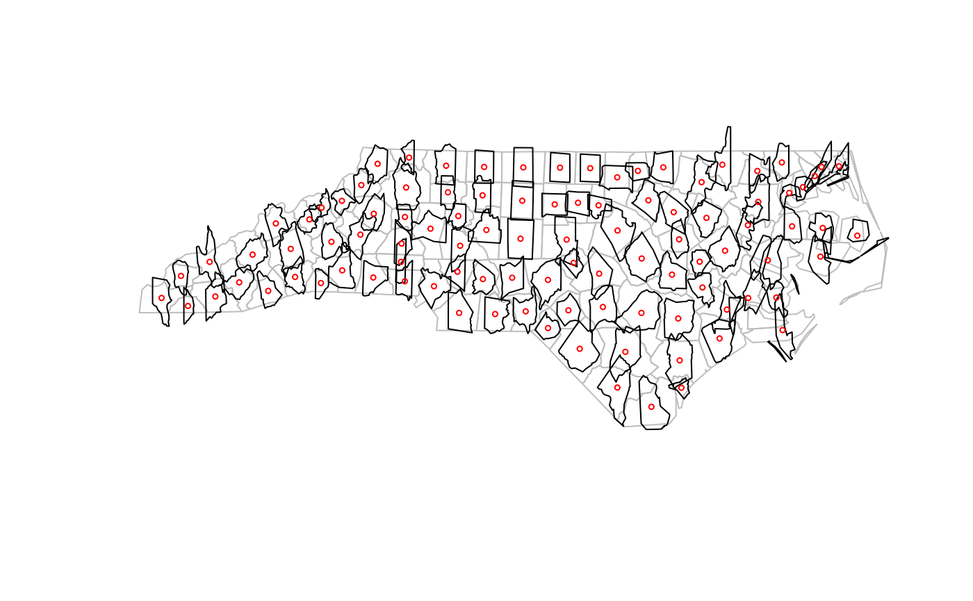

Coordinate reference systems conversion and transformation

Getting and setting coordinate reference systems of sf objects

The coordinate reference system of objects of class sfor sfc is obtained by [st_crs()](../reference/st%5Fcrs.html), and replaced by st_crs<-:

library(sf)
geom = st_sfc(st_point(c(0,1)), st_point(c(11,12)))
s = st_sf(a = 15:16, geometry = geom)
st_crs(s)
## Coordinate Reference System: NA
s1 = s
st_crs(s1) <- 4326
st_crs(s1)
## Coordinate Reference System:
##   User input: EPSG:4326 
##   wkt:
## GEOGCRS["WGS 84",
##     ENSEMBLE["World Geodetic System 1984 ensemble",
##         MEMBER["World Geodetic System 1984 (Transit)"],
##         MEMBER["World Geodetic System 1984 (G730)"],
##         MEMBER["World Geodetic System 1984 (G873)"],
##         MEMBER["World Geodetic System 1984 (G1150)"],
##         MEMBER["World Geodetic System 1984 (G1674)"],
##         MEMBER["World Geodetic System 1984 (G1762)"],
##         MEMBER["World Geodetic System 1984 (G2139)"],
##         ELLIPSOID["WGS 84",6378137,298.257223563,
##             LENGTHUNIT["metre",1]],
##         ENSEMBLEACCURACY[2.0]],
##     PRIMEM["Greenwich",0,
##         ANGLEUNIT["degree",0.0174532925199433]],
##     CS[ellipsoidal,2],
##         AXIS["geodetic latitude (Lat)",north,
##             ORDER[1],
##             ANGLEUNIT["degree",0.0174532925199433]],
##         AXIS["geodetic longitude (Lon)",east,
##             ORDER[2],
##             ANGLEUNIT["degree",0.0174532925199433]],
##     USAGE[
##         SCOPE["Horizontal component of 3D system."],
##         AREA["World."],
##         BBOX[-90,-180,90,180]],
##     ID["EPSG",4326]]
s2 = s
st_crs(s2) <- "+proj=longlat +datum=WGS84"
all.equal(s1, s2)
## [1] "Component \"geometry\": Attributes: < Component \"crs\": Component \"input\": 1 string mismatch >"
## [2] "Component \"geometry\": Attributes: < Component \"crs\": Component \"wkt\": 1 string mismatch >"

An alternative, more pipe-friendly version ofst_crs<- is

s1 %>% st_set_crs(4326)
## Simple feature collection with 2 features and 1 field
## Geometry type: POINT
## Dimension:     XY
## Bounding box:  xmin: 0 ymin: 1 xmax: 11 ymax: 12
## Geodetic CRS:  WGS 84
##    a      geometry
## 1 15   POINT (0 1)
## 2 16 POINT (11 12)

Coordinate reference system transformations

If we change the coordinate reference system from one non-missing value into another non-missing value, the CRS is is changed without modifying any coordinates, but a warning is issued that this did not reproject values:

s3 <- s1 %>% st_set_crs(4326) %>% st_set_crs(3857)
## Warning: st_crs<- : replacing crs does not reproject data; use st_transform for
## that

A cleaner way to do this that better expresses intention and does not generate this warning is to first wipe the CRS by assigning it a missing value, and then set it to the intended value.

To carry out a coordinate conversion or transformation, we use[st_transform()](../reference/st%5Ftransform.html)

s3 <- s1 %>% st_transform(3857)
s3
## Simple feature collection with 2 features and 1 field
## Geometry type: POINT
## Dimension:     XY
## Bounding box:  xmin: 0 ymin: 111325.1 xmax: 1224514 ymax: 1345708
## Projected CRS: WGS 84 / Pseudo-Mercator
##    a                geometry
## 1 15      POINT (0 111325.1)
## 2 16 POINT (1224514 1345708)

for which we see that coordinates are actually modified (projected).

Geometrical operations

All geometrical operations st_op(x) orst_op2(x,y) work both for sf objects and forsfc objects x and y; since the operations work on the geometries, the non-geometry parts of ansf object are simply discarded. Also, all binary operationsst_op2(x,y) called with a single argument, asst_op2(x), are handled as st_op2(x,x).

We will illustrate the geometrical operations on a very simple dataset:

b0 = st_polygon(list(rbind(c(-1,-1), c(1,-1), c(1,1), c(-1,1), c(-1,-1))))
b1 = b0 + 2
b2 = b0 + c(-0.2, 2)
x = st_sfc(b0, b1, b2)
a0 = b0 * 0.8
a1 = a0 * 0.5 + c(2, 0.7)
a2 = a0 + 1
a3 = b0 * 0.5 + c(2, -0.5)
y = st_sfc(a0,a1,a2,a3)
plot(x, border = 'red')
plot(y, border = 'green', add = TRUE)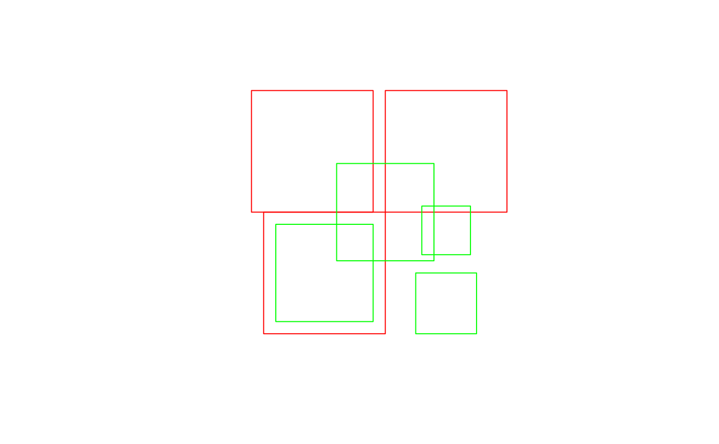

Unary operations

[st_is_valid()](../reference/valid.html) returns whether polygon geometries are topologically valid:

b0 = st_polygon(list(rbind(c(-1,-1), c(1,-1), c(1,1), c(-1,1), c(-1,-1))))
b1 = st_polygon(list(rbind(c(-1,-1), c(1,-1), c(1,1), c(0,-1), c(-1,-1))))
st_is_valid(st_sfc(b0,b1))
## [1]  TRUE FALSE

and [st_is_simple()](../reference/geos%5Fquery.html) whether line geometries are simple:

s = st_sfc(st_linestring(rbind(c(0,0), c(1,1))), 
    st_linestring(rbind(c(0,0), c(1,1),c(0,1),c(1,0))))
st_is_simple(s)
## [1]  TRUE FALSE

[st_area()](../reference/geos%5Fmeasures.html) returns the area of polygon geometries,[st_length()](../reference/geos%5Fmeasures.html) the length of line geometries:

st_area(x)
## [1] 4 4 4
st_area(st_sfc(st_point(c(0,0))))
## [1] 0
st_length(st_sfc(st_linestring(rbind(c(0,0),c(1,1),c(1,2))), st_linestring(rbind(c(0,0),c(1,0)))))
## [1] 2.414214 1.000000
st_length(st_sfc(st_multilinestring(list(rbind(c(0,0),c(1,1),c(1,2))),rbind(c(0,0),c(1,0))))) # ignores 2nd part!
## [1] 2.414214

Binary operations: distance and relate

[st_distance()](../reference/geos%5Fmeasures.html) computes the shortest distance matrix between geometries; this is a dense matrix:

st_distance(x,y)
##           [,1] [,2] [,3]     [,4]
## [1,] 0.0000000  0.6    0 0.500000
## [2,] 0.2828427  0.0    0 1.000000
## [3,] 0.2000000  0.8    0 1.220656

[st_relate()](../reference/st%5Frelate.html) returns a dense character matrix with the DE9-IM relationships between each pair of geometries:

st_relate(x,y)
##      [,1]        [,2]        [,3]        [,4]       
## [1,] "212FF1FF2" "FF2FF1212" "212101212" "FF2FF1212"
## [2,] "FF2FF1212" "212101212" "212101212" "FF2FF1212"
## [3,] "FF2FF1212" "FF2FF1212" "212101212" "FF2FF1212"

element [i,j] of this matrix has nine characters, referring to relationship between x[i] and y[j], encoded asIxIy,IxBy,IxEy,BxIy,BxBy,BxEy,ExIy,ExBy,ExEyI_xI_y,I_xB_y,I_xE_y,B_xI_y,B_xB_y,B_xE_y,E_xI_y,E_xB_y,E_xE_ywhereIIrefers to interior,BBto boundary, andEEto exterior, and e.g. BxIyB_xI_ythe dimensionality of the intersection of the the boundaryBxB_xof x[i] and the interiorIyI_yof y[j], which is one of {0,1,2,F}, indicating zero-, one-, two-dimension intersection, and (F) no intersection, respectively.

Binary logical operations:

Binary logical operations return either a sparse matrix

st_intersects(x,y)
## Sparse geometry binary predicate list of length 3, where the predicate
## was `intersects'
##  1: 1, 3
##  2: 2, 3
##  3: 3

or a dense matrix

st_intersects(x, x, sparse = FALSE)
##      [,1]  [,2]  [,3]
## [1,] TRUE  TRUE  TRUE
## [2,] TRUE  TRUE FALSE
## [3,] TRUE FALSE  TRUE
st_intersects(x, y, sparse = FALSE)
##       [,1]  [,2] [,3]  [,4]
## [1,]  TRUE FALSE TRUE FALSE
## [2,] FALSE  TRUE TRUE FALSE
## [3,] FALSE FALSE TRUE FALSE

where list element i of a sparse matrix contains the indices of the TRUE elements in row i of the the dense matrix. For large geometry sets, dense matrices take up a lot of memory and are mostly filled with FALSE values, hence the default is to return a sparse matrix.

[st_intersects()](../reference/geos%5Fbinary%5Fpred.html) returns for every geometry pair whether they intersect (dense matrix), or which elements intersect (sparse). Note that [st_intersection()](../reference/geos%5Fbinary%5Fops.html) in this package returns a geometry for the intersection instead of logicals as in[st_intersects()](../reference/geos%5Fbinary%5Fpred.html) (see the next section of this vignette).

Other binary predicates include (using sparse for readability):

st_disjoint(x, y, sparse = FALSE)
##       [,1]  [,2]  [,3] [,4]
## [1,] FALSE  TRUE FALSE TRUE
## [2,]  TRUE FALSE FALSE TRUE
## [3,]  TRUE  TRUE FALSE TRUE
st_touches(x, y, sparse = FALSE)
##       [,1]  [,2]  [,3]  [,4]
## [1,] FALSE FALSE FALSE FALSE
## [2,] FALSE FALSE FALSE FALSE
## [3,] FALSE FALSE FALSE FALSE
st_crosses(s, s, sparse = FALSE)
##       [,1]  [,2]
## [1,] FALSE FALSE
## [2,] FALSE FALSE
st_within(x, y, sparse = FALSE)
##       [,1]  [,2]  [,3]  [,4]
## [1,] FALSE FALSE FALSE FALSE
## [2,] FALSE FALSE FALSE FALSE
## [3,] FALSE FALSE FALSE FALSE
st_contains(x, y, sparse = FALSE)
##       [,1]  [,2]  [,3]  [,4]
## [1,]  TRUE FALSE FALSE FALSE
## [2,] FALSE FALSE FALSE FALSE
## [3,] FALSE FALSE FALSE FALSE
st_overlaps(x, y, sparse = FALSE)
##       [,1]  [,2] [,3]  [,4]
## [1,] FALSE FALSE TRUE FALSE
## [2,] FALSE  TRUE TRUE FALSE
## [3,] FALSE FALSE TRUE FALSE
st_equals(x, y, sparse = FALSE)
##       [,1]  [,2]  [,3]  [,4]
## [1,] FALSE FALSE FALSE FALSE
## [2,] FALSE FALSE FALSE FALSE
## [3,] FALSE FALSE FALSE FALSE
st_covers(x, y, sparse = FALSE)
##       [,1]  [,2]  [,3]  [,4]
## [1,]  TRUE FALSE FALSE FALSE
## [2,] FALSE FALSE FALSE FALSE
## [3,] FALSE FALSE FALSE FALSE
st_covered_by(x, y, sparse = FALSE)
##       [,1]  [,2]  [,3]  [,4]
## [1,] FALSE FALSE FALSE FALSE
## [2,] FALSE FALSE FALSE FALSE
## [3,] FALSE FALSE FALSE FALSE
st_covered_by(y, y, sparse = FALSE)
##       [,1]  [,2]  [,3]  [,4]
## [1,]  TRUE FALSE FALSE FALSE
## [2,] FALSE  TRUE FALSE FALSE
## [3,] FALSE FALSE  TRUE FALSE
## [4,] FALSE FALSE FALSE  TRUE
st_equals_exact(x, y,0.001, sparse = FALSE)
##       [,1]  [,2]  [,3]  [,4]
## [1,] FALSE FALSE FALSE FALSE
## [2,] FALSE FALSE FALSE FALSE
## [3,] FALSE FALSE FALSE FALSE

Operations returning a geometry

par(mfrow=c(1,2), mar = rep(0,4))
plot(st_buffer(u, 0.2))
plot(u, border = 'red', add = TRUE)
plot(st_buffer(u, 0.2), border = 'grey')
plot(u, border = 'red', add = TRUE)
plot(st_buffer(u, -0.2), add = TRUE)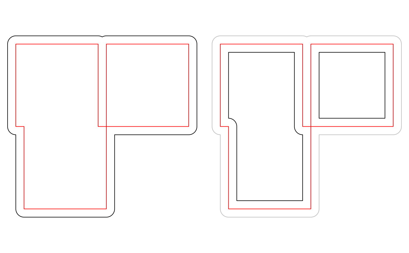

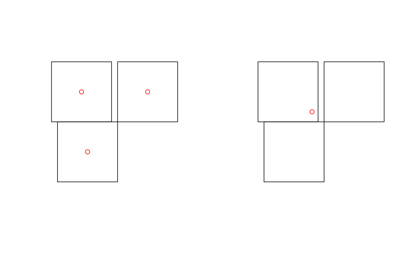
The intersection of two geometries is the geometry covered by both; it is obtained by [st_intersection()](../reference/geos%5Fbinary%5Fops.html):

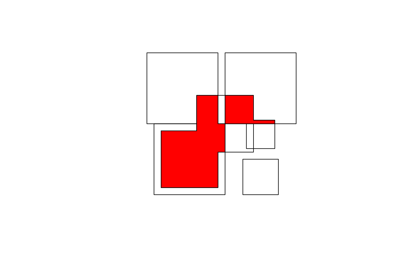
Note that [st_intersects()](../reference/geos%5Fbinary%5Fpred.html) returns a logical matrix indicating whether each geometry pair intersects (see the previous section in this vignette).

To get everything but the intersection, use[st_difference()](../reference/geos%5Fbinary%5Fops.html) or [st_sym_difference()](../reference/geos%5Fbinary%5Fops.html):

par(mfrow=c(2,2), mar = c(0,0,1,0))
plot(x, col = '#ff333388'); 
plot(y, add=TRUE, col='#33ff3388')
title("x: red, y: green")
plot(x, border = 'grey')
plot(st_difference(st_union(x),st_union(y)), col = 'lightblue', add = TRUE)
title("difference(x,y)")
plot(x, border = 'grey')
plot(st_difference(st_union(y),st_union(x)), col = 'lightblue', add = TRUE)
title("difference(y,x)")
plot(x, border = 'grey')
plot(st_sym_difference(st_union(y),st_union(x)), col = 'lightblue', add = TRUE)
title("sym_difference(x,y)")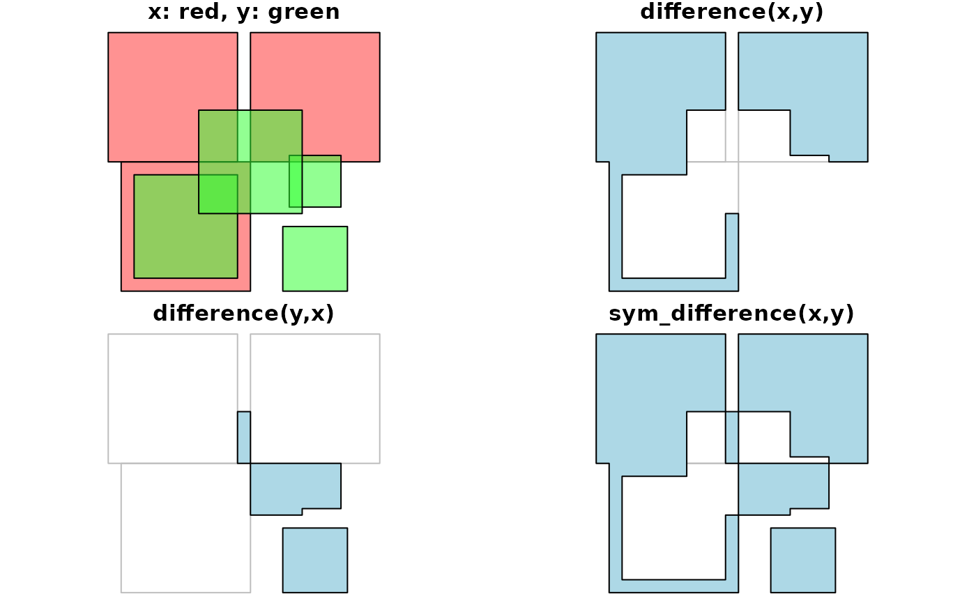

[st_segmentize()](../reference/geos%5Funary.html) adds points to straight line sections of a lines or polygon object:

par(mfrow=c(1,3),mar=c(1,1,0,0))
pts = rbind(c(0,0),c(1,0),c(2,1),c(3,1))
ls = st_linestring(pts)
plot(ls)
points(pts)
ls.seg = st_segmentize(ls, 0.3)
plot(ls.seg)
pts = ls.seg
points(pts)
pol = st_polygon(list(rbind(c(0,0),c(1,0),c(1,1),c(0,1),c(0,0))))
pol.seg = st_segmentize(pol, 0.3)
plot(pol.seg, col = 'grey')
points(pol.seg[[1]])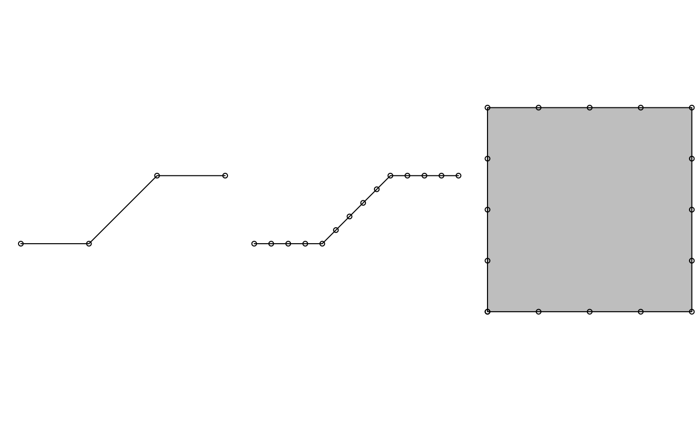

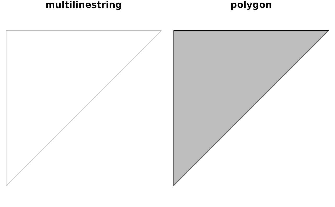
[st_polygonize()](../reference/geos%5Funary.html) polygonizes a multilinestring, as long as the points form a closed polygon:

par(mfrow=c(1,2),mar=c(0,0,1,0))
mls = st_multilinestring(list(matrix(c(0,0,0,1,1,1,0,0),,2,byrow=TRUE)))
x = st_polygonize(mls)
plot(mls, col = 'grey')
title("multilinestring")
plot(x, col = 'grey')
title("polygon")