Getting started with R (original) (raw)

Introduction

This tutorial shows how to get started with R and it specifically focuses on R for analyzing language data but it offers valuable information for anyone who wants to get started with R. As such, this tutorial is aimed at fresh users or beginners with the aim of showcasing how to set up a R session in RStudio, how to set up R projects, and how to do basic operations using R. The aim is not to provide a fully-fledged from beginner-to-expert, all-you-need-to-know tutorial but rather to show how to properly and tidily set up a project before you start coding and exemplify common operations such as loading and manipulation tabular data and generating basic visualization using R.

The entire R Notebook for the tutorial can be downloaded here. If you want to render the R Notebook on your machine, i.e. knitting the document to html or a pdf, you need to make sure that you have R and RStudio installed and you also need to download the bibliography file and store it in the same folder where you store the Rmd or the Rproj file.

Here is an overview of cheat sheets for popular and frequently used packages providde by RStudio (cheat sheets are short overviews with explanations and examples of useful functions). If you already have experience with R, both Wickham and Grolemund (2016) (see here) and Gillespie and Lovelace (2016) (see here) are highly recommendable and excellent resources for improving your coding abilities and workflows in R.

Goals of this tutorial

The goals of this tutorial are:

How to get started with R
How to orient yourself to R and RStudio
How to create and work in R projects
How to know where to look for help and to learn more about R
Understand the basics of working with data: load data, save data, working with tables, create a simple plot
Learn some best practices for using R scripts, using data, and projects
Understand the basics of objects, functions, and indexing

Audience

The intended audience for this tutorial is beginner-level, with no previous experience using R. Thus, no prior knowledge of R is required.

If you want to know more, would like to get some more practice, or would like to have another approach to R, please check out the workshops and resources on R provided by the UQ library. In addition, there are various online resources available to learn R (you can check out a very recommendable introduction here).

Installing R and RStudio

You have NOT yet installed R on your computer?
- You have a Windows computer? Then click herefor downloading and installing R
- You have a Mac? Then click here for downloading and installing R
You have NOT yet installed RStudio on your computer?
- Click herefor downloading and installing RStudio.

You can find a more elaborate explanation of how to download and install R and RStudio herethat was created by the UQ library.

Preparation

Before you actually open R or RStudio, there things to consider that make working in R much easier and give your workflow a better structure.

Imagine it like this: when you want to write a book, you could simply take pen and paper and start writing or you could think about what you want to write about, what different chapters your book would consist of, which chapters to write first, what these chapters will deal with, etc. The same is true for R: you could simply open R and start writing code or you can prepare you session and structure what you will be doing.

Folder Structure and R projects

Before actually starting with writing code, you should prepare the session by going through the following steps:

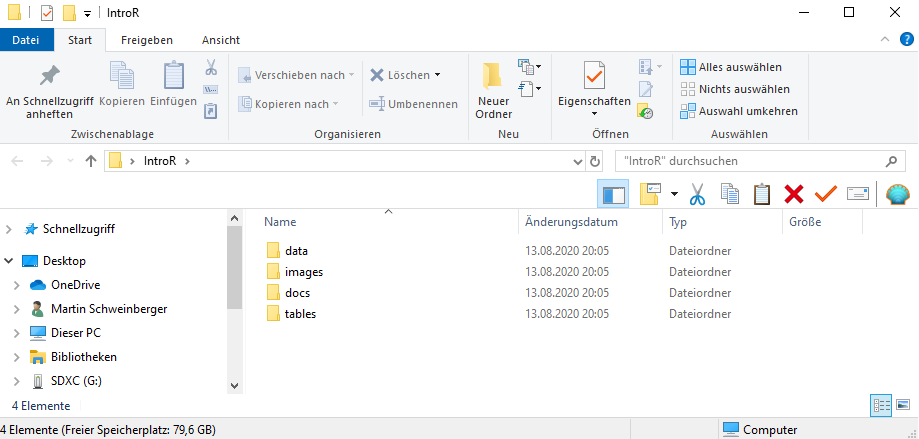
1. Create a folder for your project

In that folder, create the following sub-folders (you can, of course, adapt this folder template to match your needs)

data (you do not create this folder for the present workshop as you can simply use the data folder that you downloaded for this workshop instead)
images
tables
docs

The folder for your project could look like the the one shown below.

Once you have created your project folder, you can go ahead with RStudio.

2. Open RStudio

This is what RStudio looks like when you first open it:

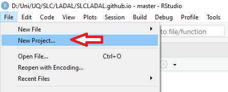
In RStudio, click on File

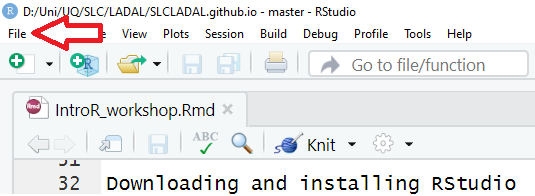
You can use the drop-down menu to create a R project

3. R Projects

In RStudio, click on New Project

Next, confirm by clicking OK and selectExisting Directory.

Then, navigate to where you have just created the project folder for this workshop.

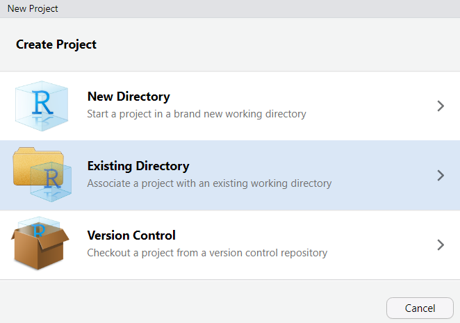
Once you click on Open, you have created a newR project

4. R Notebooks

In this project, click on File

Click on New File and then on R Notebook as shown below.

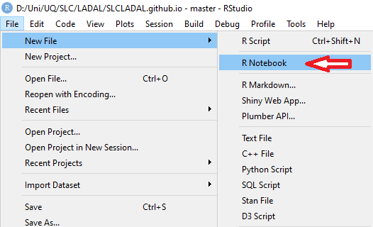
This R Notebook will be the file in which you do all your work.

5. Updating R

In case you encounter issues when opening the R Notebook (e.g., if you receive an error message saying that you need to update packages which then do not install properly), you may have to update your R version.

To update your current R version to the recent release please copy the code chunk shown below into the console pane (the bottom left pane) and click on Enter to run the code. The code will automatically update your version of R to the most recent release. During the update, you may be asked to specify some options - in that case, you can simply click on Accept and Next and accept the default settings.

# install installr package
install.packages("installr")
# load installr package
library(installr)
# update r
updateR()

6. Optimizing R project options

When you work with projects, it is recommendable to control the so-called environment. This means that you make your R Project self-contained by storing all packages that are used in project in a library in the R Project (instead of in the general R library on your computer). Having a library in your R Project means that you can share your project folder wit other people and they will automatically have the same package versions that you have sued which makes your code more robust and reproducible.

So, how to create such an environment? You simply click onTools (at the very top right of RStudio), then click onProject Options then click on Environmentsand then check Use renv with this project. Now, when you install packages, they will be installed in the package library (rather than the general R library on your computer).

7. Getting started with R Notebooks

You can now start writing in this R Notebook. For instance, you could start by changing the title of the R Notebook and describe what you are doing (what this Notebook contains).

Below is a picture of what this document looked like when I started writing it.

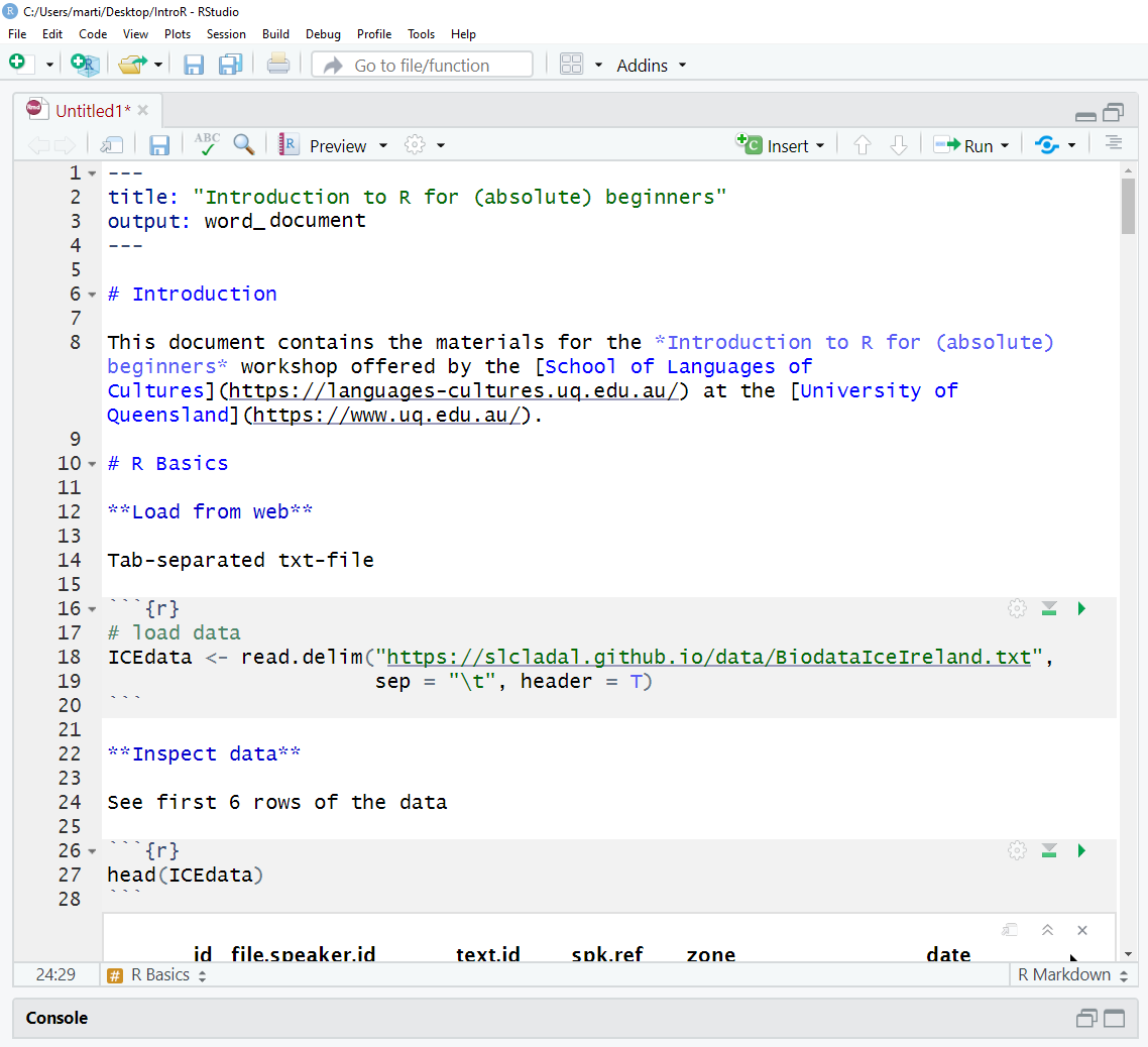
When you write in the R Notebook, you use what is calledR Markdown which is explained below.

R Markdown

The Notebook is an R Markdown document: a Rmd (R Markdown) file is more than a flat text document: it’s a program that you can run in R and which allows you to combine prose and code, so readers can see the technical aspects of your work while reading about their interpretive significance.

You can get a nice and short overview of the formatting options in R Markdown (Rmd) files here.

R Markdown allows you to make your research fully transparent and reproducible! If a couple of years down the line another researcher or a journal editor asked you how you have done your analysis, you can simply send them the Notebook or even the entire R-project folder.

As such, Rmd files are a type of document that allows to

include snippets of code (and any outputs such as tables or graphs) in plain text while
encoding the structure of your document by using simple typographical symbols to encode formatting (rather than HTML tags or format types such as Main header or Header level 1 in Word).

Markdown is really quite simple to learn and these resources may help:

The Markdown Wikipedia page includes a very handy chart of the syntax.
John Gruber developed Markdown and his introduction to the syntax is worth browsing.
This interactive Markdown tutorial will teach you the syntax in a few minutes.

R and RStudio Basics

RStudio is a so-called IDE - Integrated Development Environment. The interface provides easy access to R. The advantage of this application is that R programs and files as well as a project directory can be managed easily. The environment is capable of editing and running program code, viewing outputs and rendering graphics. Furthermore, it is possible to view variables and data objects of an R-script directly in the interface.

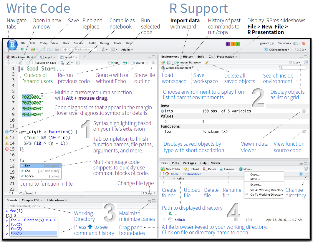
RStudio: Panes

The GUI - Graphical User Interface - that RStudio provides divides the screen into four areas that are called panes:

File editor
Environment variables
R console
Management panes (File browser, plots, help display and R packages).

The two most important are the R console (bottom left) and the File editor (or Script in the top left). The Environment variables and Management panes are on the right of the screen and they contain:

Environment (top): Lists all currently defined objects and data sets
History (top): Lists all commands recently used or associated with a project
Plots (bottom): Graphical output goes here
Help (bottom): Find help for R packages and functions. Don’t forget you can type ? before a function name in the console to get info in the Help section.
Files (bottom): Shows the files available to you in your working directory

These RStudio panes are shown below.

R Console (bottom left pane)

The console pane allows you to quickly and immediately execute R code. You can experiment with functions here, or quickly print data for viewing.

Type next to the > and press Enter to execute.

EXERCISE TIME!

You can use R like a calculator. Try typing 2+8 into the R console. Answer

2+8

  ## [1] 10

Here, the plus sign is the operator. Operators are symbols that represent some sort of action. However, R is, of course, much more than a simple calculator. To use R more fully, we need to understand objects, functions, andindexing - which we will learn about as we go.

For now, think of objects as nouns and functions as verbs.

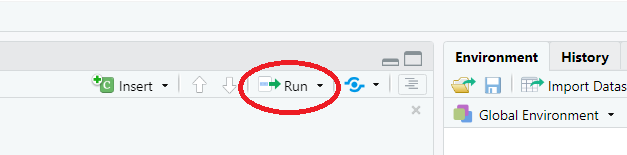
Running commands from a script

To run code from a script, insert your cursor on a line with a command, and press CTRL/CMD+Enter.

Or highlight some code to only run certain sections of the command, then press CTRL/CMD+Enter to run.

Alternatively, use the Run button at the top of the pane to execute the current line or selection (see below).

Script Editor (top left pane)

In contrast to the R console, which quickly runs code, the Script Editor (in the top left) does not automatically execute code. The Script Editor allows you to save the code essential to your analysis. You can re-use that code in the moment, refer back to it later, or publish it for replication.

Now, that we have explored RStudio, we are ready to get started with R!

This section introduces some basic concepts and procedures that help optimize your workflow in R.

Setting up an R session

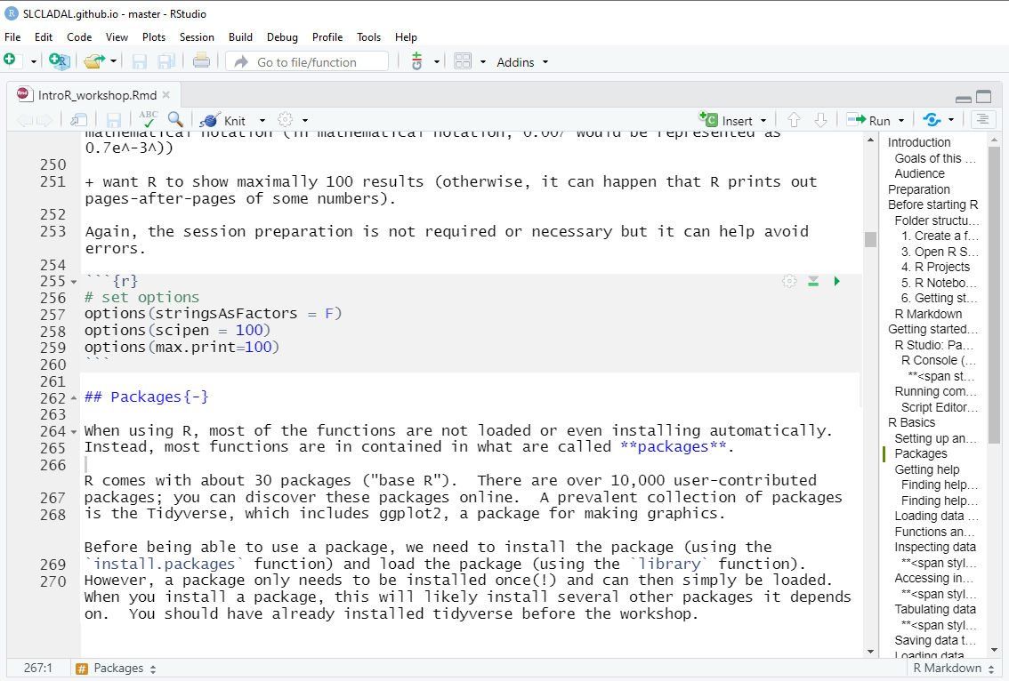
At the beginning of a session, it is common practice to define some basic parameters. This is not required or even necessary, but it may just help further down the line. This session preparation may include specifying options. In the present case, we

want R to show numbers as numbers up to 100 decimal points (and not show them in mathematical notation (in mathematical notation, 0.007 would be represented as 0.7e-3))
want R to show maximally 100 results (otherwise, it can happen that R prints out pages-after-pages of some numbers).

Again, the session preparation is not required or necessary but it can help avoid errors.

# set options
options(stringsAsFactors = F)                           
options(scipen = 100) 
options(max.print=100)

In script editor pane of RStudio, this would look like this:

Packages

When using R, most of the functions are not loaded or even installing automatically. Instead, most functions are in contained in what are called packages.

R comes with about 30 packages (“base R”). There are over 10,000 user-contributed packages; you can discover these packages online. A prevalent collection of packages is the Tidyverse, which includes ggplot2, a package for making graphics.

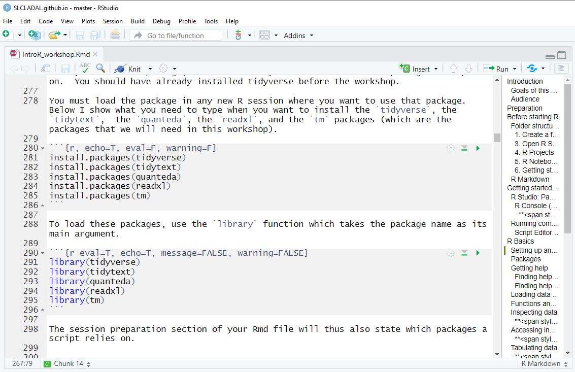
Before being able to use a package, we need to install the package (using the install.packages function) and load the package (using the library function). However, a package only needs to be installed once(!) and can then simply be loaded. When you install a package, this will likely install several other packages it depends on. You should have already installed tidyverse before the workshop.

You must load the package in any new R session where you want to use that package. Below I show what you need to type when you want to install the tidyverse, the tidytext, thequanteda, the readxl, and the tmpackages (which are the packages that we will need in this workshop).

install.packages("tidyverse")
install.packages("tidytext")
install.packages("quanteda")
install.packages("readxl")
install.packages("tm")
install.packages("tokenizers")
install.packages("here")
install.packages("flextable")
# install klippy for copy-to-clipboard button in code chunks
install.packages("remotes")
remotes::install_github("rlesur/klippy")

To load these packages, use the library function which takes the package name as its main argument.

library(tidyverse)
library(tidytext)
library(quanteda)
library(readxl)
library(tm)
library(tokenizers)
library(here)
library(flextable)
# activate klippy for copy-to-clipboard button
klippy::klippy()

The session preparation section of your Rmd file will thus also state which packages a script relies on.

In script editor pane of RStudio, the code blocks that install and activate packages would look like this:

Getting help

When working with R, you will encounter issues and face challenges. A very good thing about R is that it provides various ways to get help or find information about the issues you face.

Finding help within R

To get help regrading what functions a package contains, which arguments a function takes or to get information about how to use a function, you can use the help function or theapropos. function or you can simply type a ?before the package or two ?? if this does not give you any answers.

help(tidyverse) 
apropos("tidyverse")
?require

There are also other “official” help resources from R/RStudio.

Read official package documentation, see vignettes, e.g., Tidyverse https://cran.r-project.org/package=tidyverse
Use the RStudio Cheat Sheets at https://www.rstudio.com/resources/cheatsheets/
Use the RStudio Help viewer by typing ? before a function or package
Check out the keyboard shortcuts Help underTools in RStudio for some good tips

Working with tables

We will now start working with data in R. As most of the data that we work with comes in tables, we will focus on this first before moving on to working with text data.

Loading data from the web

To show, how data can be downloaded from the web, we will download a tab-separated txt-file. Translated to prose, the code below means_Create an object called_ icebio and in that object, store the result of the read.delim function.

read.delim stands for read delimited file and it takes the URL from which to load the data (or the path to the data on your computer) as its first argument. The sep stand for separator and the \t stands for tab-separated and represents the second argument that the read.delim function takes. The third argument, header, can take either T(RUE) or F(ALSE) and it tells R if the data has column names (headers) or not.

Functions and Objects

In R, functions always have the following form:function(argument1, argument2, ..., argumentN). Typically a function does something to an object (e.g. a table), so that the first argument typically specifies the data to which the function is applied. Other arguments then allow to add some information. Just as a side note, functions are also objects that do not contain data but instructions.

To assign content to an object, we use <- or= so that the we provide a name for an object, and then assign some content to it. For example, MyObject <- 1:3means Create an object called MyObject. this object should contain the numbers 1 to 3.

# load data
icebio <- read.delim("https://slcladal.github.io/data/BiodataIceIreland.txt", 
                      sep = "\t", header = T)

Inspecting data

There are many ways to inspect data. We will briefly go over the most common ways to inspect data.

The head function takes the data-object as its first argument and automatically shows the first 6 elements of an object (or rows if the data-object has a table format).

head(icebio)

##   id file.speaker.id text.id spk.ref             zone      date    sex   age
## 1  1     <S1A-001$A> S1A-001       A northern ireland 1990-1994   male 34-41
## 2  2     <S1A-001$B> S1A-001       B northern ireland 1990-1994 female 34-41
## 3  3     <S1A-002$?> S1A-002       ?             <NA>      <NA>   <NA>  <NA>
## 4  4     <S1A-002$A> S1A-002       A northern ireland 2002-2005 female 26-33
## 5  5     <S1A-002$B> S1A-002       B northern ireland 2002-2005 female 19-25
## 6  6     <S1A-002$C> S1A-002       C northern ireland 2002-2005   male   50+
##   word.count
## 1        765
## 2       1298
## 3         23
## 4        391
## 5         47
## 6        200

We can also use the head function to inspect more or less elements and we can specify the number of elements (or rows) that we want to inspect as a second argument. In the example below, the4 tells R that we only want to see the first 4 rows of the data.

head(icebio, 4)

##   id file.speaker.id text.id spk.ref             zone      date    sex   age
## 1  1     <S1A-001$A> S1A-001       A northern ireland 1990-1994   male 34-41
## 2  2     <S1A-001$B> S1A-001       B northern ireland 1990-1994 female 34-41
## 3  3     <S1A-002$?> S1A-002       ?             <NA>      <NA>   <NA>  <NA>
## 4  4     <S1A-002$A> S1A-002       A northern ireland 2002-2005 female 26-33
##   word.count
## 1        765
## 2       1298
## 3         23
## 4        391

EXERCISE TIME!

Download and inspect the first 7 rows of the data set that you can find under this URL:https://slcladal.github.io/data/lmmdata.txt. Can you guess what the data is about? Answer

  ex1data <- read.delim("https://slcladal.github.io/data/lmmdata.txt", sep = "\t")
  head(ex1data, 7)

  ##   Date         Genre    Text Prepositions Region
  ## 1 1736       Science   albin       166.01  North
  ## 2 1711     Education    anon       139.86  North
  ## 3 1808 PrivateLetter  austen       130.78  North
  ## 4 1878     Education    bain       151.29  North
  ## 5 1743     Education barclay       145.72  North
  ## 6 1908     Education  benson       120.77  North
  ## 7 1906         Diary  benson       119.17  North

The data is about texts and the different columns provide information about the texts such as when the texts were written (Date), the genre the texts represent (Genre), the name of the texts (Text), the relative frequencies of prepositions the texts contain (Prepositions), and the region where the author was from (Region).

Accessing individual cells in a table

If you want to access specific cells in a table, you can do so by typing the name of the object and then specify the rows and columns in square brackets (i.e. data[row, column]). For example,icebio[2, 4] would show the value of the cell in the second row and fourth column of the object icebio. We can also use the colon to define a range (as shown below, where 1:5 means from 1 to 5 and 1:3 means from 1 to 3) The command icebio[1:5, 1:3]thus means:

Show me the first 5 rows and the first 3 columns of the data-object that is called icebio.

icebio[1:5, 1:3]

##   id file.speaker.id text.id
## 1  1     <S1A-001$A> S1A-001
## 2  2     <S1A-001$B> S1A-001
## 3  3     <S1A-002$?> S1A-002
## 4  4     <S1A-002$A> S1A-002
## 5  5     <S1A-002$B> S1A-002

EXERCISE TIME!

How would you inspect the content of the cells in 4thcolumn, rows 3 to 5 of the icebio data set? Answer

  icebio[3:5, 4]

  ## [1] "?" "A" "B"

Inspecting the structure of data

You can use the str function to inspect the structure of a data set. This means that this function will show the number of observations (rows) and variables (columns) and tell you what type of variables the data consists of

int = integer
chr = character string
num = numeric
fct = factor

str(icebio)

## 'data.frame':    1332 obs. of  9 variables:
##  $ id             : int  1 2 3 4 5 6 7 8 9 10 ...
##  $ file.speaker.id: chr  "<S1A-001$A>" "<S1A-001$B>" "<S1A-002$?>" "<S1A-002$A>" ...
##  $ text.id        : chr  "S1A-001" "S1A-001" "S1A-002" "S1A-002" ...
##  $ spk.ref        : chr  "A" "B" "?" "A" ...
##  $ zone           : chr  "northern ireland" "northern ireland" NA "northern ireland" ...
##  $ date           : chr  "1990-1994" "1990-1994" NA "2002-2005" ...
##  $ sex            : chr  "male" "female" NA "female" ...
##  $ age            : chr  "34-41" "34-41" NA "26-33" ...
##  $ word.count     : int  765 1298 23 391 47 200 464 639 308 78 ...

The summary function summarizes the data.

summary(icebio)

##        id         file.speaker.id      text.id            spk.ref         
##  Min.   :   1.0   Length:1332        Length:1332        Length:1332       
##  1st Qu.: 333.8   Class :character   Class :character   Class :character  
##  Median : 666.5   Mode  :character   Mode  :character   Mode  :character  
##  Mean   : 666.5                                                           
##  3rd Qu.: 999.2                                                           
##  Max.   :1332.0                                                           
##      zone               date               sex                age           
##  Length:1332        Length:1332        Length:1332        Length:1332       
##  Class :character   Class :character   Class :character   Class :character  
##  Mode  :character   Mode  :character   Mode  :character   Mode  :character  
##                                                                             
##                                                                             
##                                                                             
##    word.count    
##  Min.   :   0.0  
##  1st Qu.:  66.0  
##  Median : 240.5  
##  Mean   : 449.9  
##  3rd Qu.: 638.2  
##  Max.   :2565.0

Tabulating data

We can use the table function to create basic tables that extract raw frequency information. The following command tells us how many instances there are of each level of the variabledate in the icebio.

TIP

In order to access specific columns of a data frame, you can first type the name of the data set followed by a $ symbol and then the name of the column (or variable).

table(icebio$date)

## 
## 1990-1994 1995-2001 2002-2005 
##       905        67       270

Alternatively, you could, of course, index the column by using its position in the data set like this: icebio[, 6] - the result of table(icebio[, 6]) andtable(icebio$date) are the same! Also note that here we leave out indexes for rows to tell R that we want all rows.

When you want to cross-tabulate columns, it is often better to use the ftable function (ftable stands for_frequency table_).

ftable(icebio$age, icebio$sex)

##        female male
##                   
## 0-18        5    7
## 19-25     163   65
## 26-33      83   36
## 34-41      35   58
## 42-49      35   97
## 50+        63  138

EXERCISE TIME!

Using the table function, how many women are in the data collected between 2002 and 2005? Answer

  table(icebio$date, icebio$sex)

  ##            
  ##             female male
  ##   1990-1994    338  562
  ##   1995-2001      4   58
  ##   2002-2005    186   84

Using the ftable function, how many men are are from northern Ireland in the data collected between 1990 and 1994? Answer

  ftable(icebio$date, icebio$zone, icebio$sex)

  ##                                     female male
  ##                                                
  ## 1990-1994 mixed between ni and roi      18   13
  ##           non-corpus speaker             7   22
  ##           northern ireland             104  289
  ##           republic of ireland          209  238
  ## 1995-2001 mixed between ni and roi       0    0
  ##           non-corpus speaker             1    1
  ##           northern ireland               2   36
  ##           republic of ireland            1   21
  ## 2002-2005 mixed between ni and roi      19    7
  ##           non-corpus speaker             7    9
  ##           northern ireland             122   41
  ##           republic of ireland           38   27

Saving data to your computer

To save tabular data on your computer, you can use thewrite.table function. This function requires the data that you want to save as its first argument, the location where you want to save the data as the second argument and the type of delimiter as the third argument.

write.table(icebio, here::here("data", "icebio.txt"), sep = "\t")

A word about paths

In the code chunk above, the sequencehere::here("data", "icebio.txt") is a handy way to define a path. A path is simply the location where a file is stored on your computer or on the internet (which typically is a server - which is just a fancy term for a computer - somewhere on the globe). Thehere function from thehere package allows to simply state in which folder a certain file is and what file you are talking about.

In this case, we want to access the file icebio (which is a txt file and thus has the appendix .txt) in the data folder. R will always start looking in the folder in which your project is stored. If you want to access a file that is stored somewhere else on your computer, you can also define the full path to the folder in which the file is. In my case, this would beD:/Uni/UQ/SLC/LADAL/SLCLADAL.github.io/data. However, as the data folder in in the folder where my Rproj file is, I only need to specify that the file is in the data folder within the folder in which my Rproj file is located.

A word about package naming

Another thing that is notable in the sequencehere::here("data", "icebio.txt") is that I specified that the here function is part of the here package. This is what I meant by writing here::here which simply means use the here function from here package (package::function). This may appear to be somewhat redundant but it happens quite frequently, that different packages have functions that have the same names. In such cases, R will simply choose the function from the package that was loaded last. To prevent R from using the wrong function, it makes sense to specify the package AND the function (as I did in the sequence here::here). I only use functions without specify the package if the function is part of base R.

Loading data from your computer

To load tabular data from within your project folder (if it is in a tab-separated txt-file) you can also use the read.delimfunction. The only difference to loading from the web is that you use a path instead of a URL. If the txt-file is in the folder called_data_ in your project folder, you would load the data as shown below.

icebio <- read.delim(here::here("data", "icebio.txt"), sep = "\t", header = T)

However, you can always just use the full path (and you must do this is the data is not in your project folder).

NOTE
You may have to change the path to the data!

icebio <- read.delim(here::here("data", "icebio.txt"), 
                      sep = "\t", header = T)

To if this has worked, we will use the head function to see first 6 rows of the data

head(icebio)

##   id file.speaker.id text.id spk.ref             zone      date    sex   age
## 1  1     <S1A-001$A> S1A-001       A northern ireland 1990-1994   male 34-41
## 2  2     <S1A-001$B> S1A-001       B northern ireland 1990-1994 female 34-41
## 3  3     <S1A-002$?> S1A-002       ?             <NA>      <NA>   <NA>  <NA>
## 4  4     <S1A-002$A> S1A-002       A northern ireland 2002-2005 female 26-33
## 5  5     <S1A-002$B> S1A-002       B northern ireland 2002-2005 female 19-25
## 6  6     <S1A-002$C> S1A-002       C northern ireland 2002-2005   male   50+
##   word.count
## 1        765
## 2       1298
## 3         23
## 4        391
## 5         47
## 6        200

Loading Excel data

To load Excel spreadsheets, you can use the read_excelfunction from the readxl package as shown below. However, it may be necessary to install and activate the readxlpackage first.

icebio <- readxl::read_excel(here::here("data", "ICEdata.xlsx"))

We now briefly check column names to see if the loading of the data has worked.

colnames(icebio)

## [1] "id"              "file.speaker.id" "text.id"         "spk.ref"        
## [5] "zone"            "date"            "sex"             "age"            
## [9] "word.count"

Loading text data

There are many functions that we can use to load text data into R. For example, we can use the readLines function as shown below.

text <- readLines(here::here("data", "text2.txt"))
# inspect first text element
text[1]

## [1] "The book is presented as a manuscript written by its protagonist, a middle-aged man named Harry Haller, who leaves it to a chance acquaintance, the nephew of his landlady. The acquaintance adds a short preface of his own and then has the manuscript published. The title of this \"real\" book-in-the-book is Harry Haller's Records (For Madmen Only)."

To load many texts, we can use a loop to read all texts in a folder as shown below. In a first step, we define the paths of the texts and then, we use the sapply function to loop over the paths and read them into R.

# define paths
paths <- list.files(here::here("data/testcorpus"), full.names = T)
# load texts
texts <- sapply(paths, function(x){ readLines(x) })
# inspect first text element
texts[1]

## $`F:/data recovery/Uni/UQ/SLC/LADAL/SLCLADAL.github.io/data/testcorpus/linguistics01.txt`
## [1] "Linguistics is the scientific study of language. It involves analysing language form language meaning and language in context. The earliest activities in the documentation and description of language have been attributed to the th-century-BC Indian grammarian Pa?ini who wrote a formal description of the Sanskrit language in his A??adhyayi."                                                                                                                                                                                                                                                                      
## [2] ""                                                                                                                                                                                                                                                                                                                                                                                                                                                                                                                                                                                                                           
## [3] "Linguists traditionally analyse human language by observing an interplay between sound and meaning. Phonetics is the study of speech and non-speech sounds and delves into their acoustic and articulatory properties. The study of language meaning on the other hand deals with how languages encode relations between entities properties and other aspects of the world to convey process and assign meaning as well as manage and resolve ambiguity. While the study of semantics typically concerns itself with truth conditions pragmatics deals with how situational context influences the production of meaning. "

A method achieving the same result which uses piping (more on what that is below) and tidyverse R code is shown below.

# define paths
texts <- list.files(here::here("data/testcorpus"), full.names = T, pattern = ".*txt") %>%
  purrr::map_chr(~ readr::read_file(.))
# inspect first text element
texts[1]

## [1] "Linguistics is the scientific study of language. It involves analysing language form language meaning and language in context. The earliest activities in the documentation and description of language have been attributed to the th-century-BC Indian grammarian Pa?ini who wrote a formal description of the Sanskrit language in his A??adhyayi.\r\n\r\nLinguists traditionally analyse human language by observing an interplay between sound and meaning. Phonetics is the study of speech and non-speech sounds and delves into their acoustic and articulatory properties. The study of language meaning on the other hand deals with how languages encode relations between entities properties and other aspects of the world to convey process and assign meaning as well as manage and resolve ambiguity. While the study of semantics typically concerns itself with truth conditions pragmatics deals with how situational context influences the production of meaning. "

Renaming, Piping, and Filtering

To rename existing columns in a table, you can use therename command which takes the table as the first argument, the new name as the second argument, the an equal sign (=), and finally, the old name es the third argument. For example, renaming a column_OldName_ as NewName in a table called _MyTable_would look like this:rename(MyTable, NewName = OldName).

Piping is done using the %>% sequence and it can be translated as and then. In the example below, we create a new object (icebio_edit) from the existing object (icebio) and then we rename the columns in the new object. When we use piping, we do not need to name the data we are using as this is provided by the previous step.

icebio_edit <- icebio %>%
  dplyr::rename(Id = id,
         FileSpeakerId = file.speaker.id,
         File = colnames(icebio)[3],
         Speaker = colnames(icebio)[4])
# inspect data
icebio_edit[1:5, 1:6]

## # A tibble: 5 × 6
##      Id FileSpeakerId File    Speaker zone             date     
##   <dbl> <chr>         <chr>   <chr>   <chr>            <chr>    
## 1     1 <S1A-001$A>   S1A-001 A       northern ireland 1990-1994
## 2     2 <S1A-001$B>   S1A-001 B       northern ireland 1990-1994
## 3     3 <S1A-002$?>   S1A-002 ?       NA               NA       
## 4     4 <S1A-002$A>   S1A-002 A       northern ireland 2002-2005
## 5     5 <S1A-002$B>   S1A-002 B       northern ireland 2002-2005

A very handy way to rename many columns simultaneously, you can use the str_to_title function which capitalizes first letter of a word. In the example below, we capitalize all first letters of the column names of our current data.

colnames(icebio_edit) <- stringr::str_to_title(colnames(icebio_edit))
# inspect data
icebio_edit[1:5, 1:6]

## # A tibble: 5 × 6
##      Id Filespeakerid File    Speaker Zone             Date     
##   <dbl> <chr>         <chr>   <chr>   <chr>            <chr>    
## 1     1 <S1A-001$A>   S1A-001 A       northern ireland 1990-1994
## 2     2 <S1A-001$B>   S1A-001 B       northern ireland 1990-1994
## 3     3 <S1A-002$?>   S1A-002 ?       NA               NA       
## 4     4 <S1A-002$A>   S1A-002 A       northern ireland 2002-2005
## 5     5 <S1A-002$B>   S1A-002 B       northern ireland 2002-2005

To remove rows based on values in columns you can use thefilter function.

icebio_edit2 <- icebio_edit %>%
  dplyr::filter(Speaker != "?",
         Zone != is.na(Zone),
         Date == "2002-2005",
         Word.count > 5)
# inspect data
head(icebio_edit2)

## # A tibble: 6 × 9
##      Id Filespeakerid File    Speaker Zone          Date  Sex   Age   Word.count
##   <dbl> <chr>         <chr>   <chr>   <chr>         <chr> <chr> <chr>      <dbl>
## 1     4 <S1A-002$A>   S1A-002 A       northern ire… 2002… fema… 26-33        391
## 2     5 <S1A-002$B>   S1A-002 B       northern ire… 2002… fema… 19-25         47
## 3     6 <S1A-002$C>   S1A-002 C       northern ire… 2002… male  50+          200
## 4     7 <S1A-002$D>   S1A-002 D       northern ire… 2002… fema… 50+          464
## 5     8 <S1A-002$E>   S1A-002 E       mixed betwee… 2002… male  34-41        639
## 6     9 <S1A-002$F>   S1A-002 F       northern ire… 2002… fema… 26-33        308

To select specific columns you can use the selectfunction.

icebio_selection <- icebio_edit2 %>%
  dplyr::select(File, Speaker, Word.count)
# inspect data
head(icebio_selection)

## # A tibble: 6 × 3
##   File    Speaker Word.count
##   <chr>   <chr>        <dbl>
## 1 S1A-002 A              391
## 2 S1A-002 B               47
## 3 S1A-002 C              200
## 4 S1A-002 D              464
## 5 S1A-002 E              639
## 6 S1A-002 F              308

You can also use the select function to remove specific columns.

icebio_selection2 <- icebio_edit2 %>%
  dplyr::select(-Id, -File, -Speaker, -Date, -Zone, -Age)
# inspect data
head(icebio_selection2)

## # A tibble: 6 × 3
##   Filespeakerid Sex    Word.count
##   <chr>         <chr>       <dbl>
## 1 <S1A-002$A>   female        391
## 2 <S1A-002$B>   female         47
## 3 <S1A-002$C>   male          200
## 4 <S1A-002$D>   female        464
## 5 <S1A-002$E>   male          639
## 6 <S1A-002$F>   female        308

Ordering data

To order data, for instance, in ascending order according to a specific column you can use the arrange function.

icebio_ordered_asc <- icebio_selection2 %>%
  dplyr::arrange(Word.count)
# inspect data
head(icebio_ordered_asc)

## # A tibble: 6 × 3
##   Filespeakerid Sex    Word.count
##   <chr>         <chr>       <dbl>
## 1 <S1B-009$D>   female          6
## 2 <S1B-005$C>   female          7
## 3 <S1B-009$C>   male            7
## 4 <S1B-020$F>   male            7
## 5 <S1B-006$G>   female          9
## 6 <S2A-050$B>   male            9

To order data in descending order you can also use thearrange function and simply add a - before the column according to which you want to order the data.

icebio_ordered_desc <- icebio_selection2 %>%
  dplyr::arrange(-Word.count)
# inspect data
head(icebio_ordered_desc)

## # A tibble: 6 × 3
##   Filespeakerid Sex    Word.count
##   <chr>         <chr>       <dbl>
## 1 <S2A-055$A>   female       2355
## 2 <S2A-047$A>   male         2340
## 3 <S2A-035$A>   female       2244
## 4 <S2A-048$A>   male         2200
## 5 <S2A-015$A>   male         2172
## 6 <S2A-054$A>   female       2113

The output shows that the female speaker in file S2A-005 with the speaker identity A has the highest word count with 2,355 words.

EXERCISE TIME!

Using the data called icebio, create a new data set called ICE_Ire_ordered and arrange the data in descending order by the number of words that each speaker has uttered. Who is the speaker with the highest word count? Answer

  ICE_Ire_ordered <- icebio %>%
  dplyr::arrange(-word.count)
  # inspect data
  head(ICE_Ire_ordered)

  ## # A tibble: 6 × 9
  ##      id file.speaker.id text.id spk.ref zone        date  sex   age   word.count
  ##   <dbl> <chr>           <chr>   <chr>   <chr>       <chr> <chr> <chr>      <dbl>
  ## 1   956 <S2A-037$A>     S2A-037 A       republic o… 1990… male  NA          2565
  ## 2   919 <S2A-016$A>     S2A-016 A       republic o… 1995… fema… 34-41       2482
  ## 3   933 <S2A-023$A>     S2A-023 A       northern i… 1990… male  50+         2367
  ## 4   992 <S2A-055$A>     S2A-055 A       northern i… 2002… fema… 42-49       2355
  ## 5   979 <S2A-047$A>     S2A-047 A       republic o… 2002… male  50+         2340
  ## 6   997 <S2A-059$A>     S2A-059 A       republic o… 1990… fema… NA          2305

Creating and changing variables

New columns are created, and existing columns can be changed, by using the mutate function. The mutate function takes two arguments (if the data does not have to be specified): the first argument is the (new) name of column that you want to create and the second is what you want to store in that column. The = tells R that the new column will contain the result of the second argument.

In the example below, we create a new column called_Texttype_.

This new column should contain

the value PrivateDialoge if _Filespeakerid_contains the sequence S1A,
the value PublicDialogue if _Filespeakerid_contains the sequence S1B,
the value UnscriptedMonologue if _Filespeakerid_contains the sequence S2A,
the value ScriptedMonologue if _Filespeakerid_contains the sequence S2B,
the value of Filespeakerid if Filespeakerid_neither contains S1A, S1B, S2A, nor_S2B.

icebio_texttype <- icebio_selection2 %>%
  dplyr::mutate(Texttype = 
                  dplyr::case_when(stringr::str_detect(Filespeakerid ,"S1A") ~ "PrivateDialoge",
                                   stringr::str_detect(Filespeakerid ,"S1B") ~ "PublicDialogue",
                                   stringr::str_detect(Filespeakerid ,"S2A") ~ "UnscriptedMonologue",
                                   stringr::str_detect(Filespeakerid ,"S2B") ~ "ScriptedMonologue",
                                   TRUE ~ Filespeakerid))
# inspect data
head(icebio_texttype)

## # A tibble: 6 × 4
##   Filespeakerid Sex    Word.count Texttype      
##   <chr>         <chr>       <dbl> <chr>         
## 1 <S1A-002$A>   female        391 PrivateDialoge
## 2 <S1A-002$B>   female         47 PrivateDialoge
## 3 <S1A-002$C>   male          200 PrivateDialoge
## 4 <S1A-002$D>   female        464 PrivateDialoge
## 5 <S1A-002$E>   male          639 PrivateDialoge
## 6 <S1A-002$F>   female        308 PrivateDialoge

If-statements

We should briefly talk about if-statements (or case_whenin the present case). The case_when function is both very powerful and extremely helpful as it allows you to assign values based on a test. As such, case_when-statements can be read as:

When/If X is the case, then do A and if X is not the case do B! (When/If -> Then -> Else)

The nice thing about ifelse orcase_when-statements is that they can be used in succession as we have done above. This can then be read as:

If X is the case, then do A, if Y is the case, then do B, else do Z

EXERCISE TIME!

1.Using the data called icebio, create a new data set called ICE_Ire_AgeGroup in which you create a column calledAgeGroup where all speakers who are younger than 42 have the value young and all speakers aged 42 and over_old_.

Tip: use if-statements to assign the _old_and young values.

Answer

  ICE_Ire_AgeGroup <- icebio %>%
  dplyr::mutate(AgeGroup = dplyr::case_when(age == "42-49" ~ "old",
                                            age == "50+" ~ "old", 
                                            age == "0-18" ~ "young",
                                            age == "19-25" ~ "young",
                                            age == "26-33" ~ "young",
                                            age == "34-41" ~ "young", 
                                            TRUE ~age))
  # inspect data
  head(ICE_Ire_AgeGroup); table(ICE_Ire_AgeGroup$AgeGroup)

  ## # A tibble: 6 × 10
  ##      id file.speaker.id text.id spk.ref zone        date  sex   age   word.count
  ##   <dbl> <chr>           <chr>   <chr>   <chr>       <chr> <chr> <chr>      <dbl>
  ## 1     1 <S1A-001$A>     S1A-001 A       northern i… 1990… male  34-41        765
  ## 2     2 <S1A-001$B>     S1A-001 B       northern i… 1990… fema… 34-41       1298
  ## 3     3 <S1A-002$?>     S1A-002 ?       NA          NA    NA    NA            23
  ## 4     4 <S1A-002$A>     S1A-002 A       northern i… 2002… fema… 26-33        391
  ## 5     5 <S1A-002$B>     S1A-002 B       northern i… 2002… fema… 19-25         47
  ## 6     6 <S1A-002$C>     S1A-002 C       northern i… 2002… male  50+          200
  ## # ℹ 1 more variable: AgeGroup <chr>

  ## 
  ##    NA   old young 
  ##   547   333   452

Summarizing data

Summarizing is really helpful and can be done using thesummarise function.

icebio_summary1 <- icebio_texttype %>%
  dplyr::summarise(Words = sum(Word.count))
# inspect data
head(icebio_summary1)

## # A tibble: 1 × 1
##    Words
##    <dbl>
## 1 141876

To get summaries of sub-groups or by variable level, we can use thegroup_by function and then use the summarisefunction.

icebio_summary2 <- icebio_texttype %>%
  dplyr::group_by(Texttype, Sex) %>%
  dplyr::summarise(Speakers = n(),
            Words = sum(Word.count))
# inspect data
head(icebio_summary2)

## # A tibble: 6 × 4
## # Groups:   Texttype [3]
##   Texttype            Sex    Speakers Words
##   <chr>               <chr>     <int> <dbl>
## 1 PrivateDialoge      female      105 60024
## 2 PrivateDialoge      male         18  9628
## 3 PublicDialogue      female       63 24647
## 4 PublicDialogue      male         41 16783
## 5 UnscriptedMonologue female        3  6712
## 6 UnscriptedMonologue male         16 24082

EXERCISE TIME!

Use the icebio and determine the number of words uttered by female speakers from Northern Ireland above an age of 50. Answer

  words_fni50 <- icebio %>%
  dplyr::select(zone, sex, age, word.count) %>%
  dplyr::group_by(zone, sex, age) %>%
  dplyr::summarize(Words = sum(word.count)) %>%
  dplyr::filter(sex == "female",
         age == "50+",
         zone == "northern ireland")

  ## `summarise()` has grouped output by 'zone', 'sex'. You can override using the
  ## `.groups` argument.

  # inspect data
  words_fni50

  ## # A tibble: 1 × 4
  ## # Groups:   zone, sex [1]
  ##   zone             sex    age   Words
  ##   <chr>            <chr>  <chr> <dbl>
  ## 1 northern ireland female 50+   23210

Load the file exercisedata.txt and determine the mean scores of groups A and B.

Tip: to extract the mean, combine thesummary function with the mean function.

Answer

  exercisedata <- read.delim(here::here("data", "exercisedata.txt"), sep = "\t", header = T) %>%
  dplyr::group_by(Group) %>%
  dplyr::summarize(Mean = mean(Score))
  # inspect data
  exercisedata

  ## # A tibble: 2 × 2
  ##   Group  Mean
  ##   <chr> <dbl>
  ## 1 A      14.9
  ## 2 B      11.8

Gathering and spreading data

The tidyr package has two very useful functions for gathering and spreading data that can be sued to transform data to long and wide formats (you will see what this means below). The functions are called gather and spread.

We will use the data set called icebio_summary2, which we created above, to demonstrate how this works.

We will first check out the spread-function to create different columns for women and men that show how many of them are represented in the different text types.

icebio_summary_wide <- icebio_summary2 %>%
  dplyr::select(-Words) %>%
  tidyr::spread(Sex, Speakers)
# inspect
icebio_summary_wide

## # A tibble: 3 × 3
## # Groups:   Texttype [3]
##   Texttype            female  male
##   <chr>                <int> <int>
## 1 PrivateDialoge         105    18
## 2 PublicDialogue          63    41
## 3 UnscriptedMonologue      3    16

The data is now in what is called a wide-format as values are distributed across columns.

To reformat this back to a long-format where each column represents exactly one variable, we use thegather-function:

icebio_summary_long <- icebio_summary_wide %>%
  tidyr::gather(Sex, Speakers, female:male)
# inspect
icebio_summary_long

## # A tibble: 6 × 3
## # Groups:   Texttype [3]
##   Texttype            Sex    Speakers
##   <chr>               <chr>     <int>
## 1 PrivateDialoge      female      105
## 2 PublicDialogue      female       63
## 3 UnscriptedMonologue female        3
## 4 PrivateDialoge      male         18
## 5 PublicDialogue      male         41
## 6 UnscriptedMonologue male         16

More on working with text

We have now worked though how to load, save, and edit tabulated data. However, R is also perfectly equipped for working with textual data which is what we going to concentrate on now.

Loading text data

To load text data from the web, we can use the read_filefunction which takes the URL of the text as its first argument. In this case will will load the 2016 rally speeches Donald Trump.

Trump <-base::readRDS(url("https://slcladal.github.io/data/Trump.rda", "rb"))
# inspect data
str(Trump)

## 'data.frame':    2694 obs. of  1 variable:
##  $ SPEECH: chr  "...Thank you so much.  That's so nice.  Isn't he a great guy.  He doesn't get a fair press; he doesn't get it. "| __truncated__ "With that said, our country is really headed in the wrong direction with a president who is doing an absolutely"| __truncated__ "And I'm a conservative, actually very conservative, and I'm a Republican.  And I'm very disappointed by our Rep"| __truncated__ "You look at Obamacare.  A total catastrophe and by the way it really kicks in in '16 and it is going to be a di"| __truncated__ ...

It is very easy to extract frequency information and to create frequency lists. We can do this by first using theunnest_tokens function which splits texts into individual words, an then use the count function to get the raw frequencies of all word types in a text.

Trump %>%
  tibble(text = SPEECH) %>%
  unnest_tokens(word, text) %>%
  dplyr::count(word, sort=T)

## # A tibble: 6,102 × 2
##    word      n
##    <chr> <int>
##  1 the    5924
##  2 to     5460
##  3 and    5438
##  4 i      4873
##  5 a      3592
##  6 you    3055
##  7 of     2953
##  8 we     2565
##  9 it     2421
## 10 that   2317
## # ℹ 6,092 more rows

Extracting N-grams is also very easy as theunnest_tokens function can an argument calledtoken in which we can specify that we want to extract n-grams, If we do this, then we need to specify the n as a separate argument. Below we specify that we want the frequencies of all 4-grams.

Trump %>%
  tibble(text = SPEECH) %>%
  unnest_tokens(word, text, token="ngrams", n=4) %>%
  dplyr::count(word, sort=T) %>%
  head(10)

## # A tibble: 10 × 2
##    word                    n
##    <chr>               <int>
##  1 and we’re going to     93
##  2 we are going to        75
##  3 <NA>                   68
##  4 it’s going to be       65
##  5 we’re going to do      61
##  6 we’re going to have    61
##  7 not going to happen    60
##  8 and by the way         53
##  9 thank you very much    52
## 10 we’re going to win     50

Splitting-up texts

We can use the str_split function to split texts. However, there are two issues when using this (very useful) function:

the pattern that we want to split on disappears
the output is a list (a special type of data format)

To remedy these issues, we

combine the str_split function with theunlist function
add something right at the beginning of the pattern that we use to split the text. To add something to the beginning of the pattern that we want to split the text by, we use the str_replace_allfunction. The str_replace_all function takes three arguments, 1. the text, 2. the patternthat should be replaced, 3. the replacement. In the example below, we add ~~~ to the sequenceSPEECH and then split on the ~~~ rather than on the sequence “SPEECH” (in other words, we replace SPEECHwith ~~~SPEECH and then split on~~~).

Trump_split <- unlist(str_split(
  stringr::str_replace_all(Trump, "SPEECH", "~~~SPEECH"),
  pattern = "~~~"))
# inspect data
nchar(Trump_split)#; str(Trump_split)

##  [1]  21311  26963   2701   6004   1342  32880  28497 425099   1404 311770
## [11]  43776

Cleaning texts

When working with texts, we usually need to clean the data. Below, we do some very basic cleaning using a pipeline.

Trump_split_clean <- Trump_split %>%
  # replace elements
  stringr::str_replace_all(fixed("\n"), " ") %>%
  # remove strange symbols
  stringr::str_replace_all("[^[:alnum:][:punct:]]+", " ") %>%
  # combine contractions
  stringr::str_replace_all(" re ", "'re ") %>%
  stringr::str_replace_all(" ll ", "'ll ") %>%
  stringr::str_replace_all(" d ", "'d ") %>%
  stringr::str_replace_all(" m ", "'m ") %>%
  stringr::str_replace_all(" s ", "'s ") %>%
  stringr::str_replace_all("n t ", "n't ") %>%
  # remove \"
  stringr::str_remove_all("\"") %>%
  # remove superfluous white spaces
  stringr::str_squish()
# remove very short elements
Trump_split_clean <- Trump_split_clean[nchar(Trump_split_clean) > 5]
# inspect data
nchar(Trump_split_clean)

##  [1]  20878  26754   2687   5960   1321  32539  28303 422165   1404 309275
## [11]  43477

Inspect text

Trump_split_clean[5]

Concordancing and KWICs

Creating concordances or key-word-in-context displays is one of the most common practices when dealing with text data. Fortunately, there exist ready-made functions that make this a very easy task in R. We will use the kwic function from the quantedapackage to create kwics here.

kwic_multiple <- quanteda::kwic(Trump_split_clean, 
       pattern = phrase("great again"),
       window = 3, 
       valuetype = "regex") %>%
  as.data.frame()
# inspect data
head(kwic_multiple)

##   docname from   to               pre     keyword            post     pattern
## 1   text1 3043 3044  make our country great again       . We have great again
## 2   text1 4457 4458   to make America great again        . We can great again
## 3   text1 4465 4466 make this country great again . The potential great again
## 4   text2 5329 5330 will make America great again        . And if great again
## 5   text4  619  620   to make America great again       , folks , great again
## 6   text4  634  635   to make America great again         . , And great again

We can now also select concordances based on specific features. For example, we only want those instances of “great again” if the preceding word was “america”.

kwic_multiple_select <- kwic_multiple %>%
  # last element before search term is "america"
  dplyr::filter(str_detect(pre, "america$"))
# inspect data
head(kwic_multiple_select)

## [1] docname from    to      pre     keyword post    pattern
## <0 rows> (or 0-length row.names)

Again, we can use the write.table function to save our kwics to disc.

write.table(kwic_multiple_select, here::here("data", "kwic_multiple_select.txt"), sep = "\t")

As most of the data that we use is on out computers (rather than being somewhere on the web), we now load files with text from your computer. It is important to note that you need to use \\when you want to load data from a Windows PC (rather than single\).

To load many files, we first create a list of all files in a the directory that we want to load data from and then use thesapply function (which works just like a loop). Thesapply function takes a a vector of elements and then performs a sequence of steps on each of these elements. In the example below, we feed the file locations to the sapply function and then we scan each text (i.e. we read it into R), then we paste all the content of one file together.

NOTE
You may have to change the path to the data!

files <- list.files(here::here("data", "ICEIrelandSample"),
                    pattern = ".txt", full.names = T)
ICE_Ire_sample <- sapply(files, function(x) {
  x <- scan(x, what = "char")
  x <- paste(x, sep = " ", collapse = " ")
  })
# inspect data
str(ICE_Ire_sample)

##  Named chr [1:100] "<S1A-001 Riding> <I> <S1A-001$A> <#> Well how did the riding go tonight <S1A-001$B> <#> It was good so it was <#> Just I I coul ...
##  - attr(*, "names")= chr [1:100] "F:/data recovery/Uni/UQ/SLC/LADAL/SLCLADAL.github.io/data/ICEIrelandSample/S1A-001.txt" "F:/data recovery/Uni/UQ/SLC/LADAL/SLCLADAL.github.io/data/ICEIrelandSample/S1A-002.txt" "F:/data recovery/Uni/UQ/SLC/LADAL/SLCLADAL.github.io/data/ICEIrelandSample/S1A-003.txt" "F:/data recovery/Uni/UQ/SLC/LADAL/SLCLADAL.github.io/data/ICEIrelandSample/S1A-004.txt" ...

As the texts do not have column names (but simply names), we can clean these by removing everything before a / and by removing the .txt.

names(ICE_Ire_sample) <- names(ICE_Ire_sample) %>%
  stringr::str_remove_all(".*/") %>%
  stringr::str_remove_all(".txt")
# inspect
names(ICE_Ire_sample)

##   [1] "S1A-001"                     "S1A-002"                    
##   [3] "S1A-003"                     "S1A-004"                    
##   [5] "S1A-005"                     "S1A-006"                    
##   [7] "S1A-007"                     "S1A-008"                    
##   [9] "S1A-009"                     "S1A-010"                    
##  [11] "S1A-011"                     "S1A-012"                    
##  [13] "S1A-013"                     "S1A-014"                    
##  [15] "S1A-015"                     "S1A-016"                    
##  [17] "S1A-017"                     "S1A-018"                    
##  [19] "S1A-019"                     "S1A-020"                    
##  [21] "S1A-021"                     "S1A-022"                    
##  [23] "S1A-023"                     "S1A-024"                    
##  [25] "S1A-025"                     "S1A-026"                    
##  [27] "S1A-027"                     "S1A-028"                    
##  [29] "S1A-029"                     "S1A-030"                    
##  [31] "S1A-031"                     "S1A-032"                    
##  [33] "S1A-033"                     "S1A-034"                    
##  [35] "S1A-035"                     "S1A-036"                    
##  [37] "S1A-037"                     "S1A-038"                    
##  [39] "S1A-039"                     "S1A-040"                    
##  [41] "S1A-041"                     "S1A-042"                    
##  [43] "S1A-043"                     "S1A-044"                    
##  [45] "S1A-045"                     "S1A-046"                    
##  [47] "S1A-047"                     "S1A-048"                    
##  [49] "S1A-049"                     "S1A-050"                    
##  [51] "S1A-051"                     "S1A-052 Buttermilk"         
##  [53] "S1A-053 Student grants 1"    "S1A-054 Student grants 2"   
##  [55] "S1A-055 Hospitals"           "S1A-056 Holistic medicine 1"
##  [57] "S1A-057 Studying 2"          "S1A-058 Holistic medicine 2"
##  [59] "S1A-059 Glasses 1"           "S1A-060 Glasses 2"          
##  [61] "S1A-061 Modern man"          "S1A-062 America trip 1"     
##  [63] "S1A-063 Shoes"               "S1A-064 O'Connell Street"   
##  [65] "S1A-065 America trip 2"      "S1A-066 Radio music"        
##  [67] "S1A-067 Apprenticeship"      "S1A-068 Rock bands"         
##  [69] "S1A-069 Christmas trees"     "S1A-070 Friends"            
##  [71] "S1A-071 Elocution"           "S1A-072 Driver's licence"   
##  [73] "S1A-073 Politics"            "S1A-074 Local shops"        
##  [75] "S1A-075 Present"             "S1A-076 Boyfriends 2"       
##  [77] "S1A-077 Books"               "S1A-078 Medical project"    
##  [79] "S1A-079 Driving"             "S1A-080 Motorbikes"         
##  [81] "S1A-081 Croke Park"          "S1A-082 Kissogram"          
##  [83] "S1A-083 Donkey story"        "S1A-084 General election"   
##  [85] "S1A-085 Birthday cake"       "S1A-086 Baby"               
##  [87] "S1A-087 Line dancing"        "S1A-088 Therapy inaugural"  
##  [89] "S1A-089 American men"        "S1A-090 Designer clothes"   
##  [91] "S1A-091 Haircut - Mortgage"  "S1A-092 Househunting"       
##  [93] "S1A-093 Motorbikes"          "S1A-094 Health"             
##  [95] "S1A-095 Strep infection"     "S1A-096 Sisters 1"          
##  [97] "S1A-097 Sisters 2"           "S1A-098 Bad weather"        
##  [99] "S1A-099 Dresses"             "S1A-100 College plans"

Further splitting of texts

To split the texts into speech units where each speech unit begins with the speaker that has uttered it, we again use thesapply function.

ICE_Ire_split <- as.vector(unlist(sapply(ICE_Ire_sample, function(x){
 x <- as.vector(str_split(str_replace_all(x, "(<S1A-)", "~~~\\1"), "~~~"))  
})))
# inspect
head(ICE_Ire_split)

## [1] ""                                                                                                                                                                                    
## [2] "<S1A-001 Riding> <I> "                                                                                                                                                               
## [3] "<S1A-001$A> <#> Well how did the riding go tonight "                                                                                                                                 
## [4] "<S1A-001$B> <#> It was good so it was <#> Just I I couldn't believe that she was going to let me jump <,> that was only the fourth time you know <#> It was great <&> laughter </&> "
## [5] "<S1A-001$A> <#> What did you call your horse "                                                                                                                                       
## [6] "<S1A-001$B> <#> I can't remember <#> Oh Mary s Town <,> oh\n"

Basics of regular expressions

Next, we extract the File and the Speaker and combine Text, File, and Speaker in a table.

We use this to show the power of regular expressions(to learn more about regular expression, have a look at this very recommendable tutorial). Regular expressions are symbols or sequences of symbols that stand for

symbols or patterns (e.g. [a-z] stands for any lowercase character)
the frequency of symbols or patterns (e.g. {1,3} stands for between 1 and 3)
classes of symbols (e.g. [:punct:] stands for any punctuation symbol)
structural properties (e.g. [^[:blank:]] stands for any non-space character, \t stands for tab-stop and\n stands for a line break)

We can not go into any detail here and only touch upon the power of regular expressions.

The symbol . is one of the most powerful and most universal regular expressions as it represents (literally) any symbol or character and it thus stands for a pattern. The * is a regular expression that refers to the frequency of a pattern and it stands for 0 to an infinite number of instances. Thus, .*stands for 0 to an infinite number of any character. You can find an overview of the regular expressions that you can use in R here.

Also, if you put patterns in round brackets, R will remember the sequence within brackets and you can paste it back into a string from memory when you replace something.

When referring to symbols that are used a regular expressions such as\ or \$, you need to inform R that you actually mean the real symbol and not the regular expression and you do that by typing two \\ before the sequence in question. Have a look at the example below and try to see what the regular expressions (.*(S1A-[0-9]{3,3}).*, \n, and.*\\$([A-Z]{1,2}\\?{0,1})>.*) stand for.

ICE_Ire_split_tb <- ICE_Ire_split %>%
  as.data.frame()
# add column names
colnames(ICE_Ire_split_tb)[1] <- "Text"
# add file and speaker
ICE_Ire_split_tb <- ICE_Ire_split_tb %>%
  dplyr::filter(!str_detect(Text, "<I>"),
         Text != "") %>%
  dplyr::mutate(File = str_replace_all(Text, ".*(S1A-[0-9]{3,3}).*", "\\1"),
         File = str_remove_all(File, "\\\n"),
         Speaker = str_replace_all(Text, ".*\\$([A-Z]{1,2}\\?{0,1})>.*", "\\1"),
         Speaker = str_remove_all(Speaker, "\\\n"))

Text	File	Speaker
<S1A-001$A> <#> Well how did the riding go tonight	S1A-001	A
<S1A-001$B> <#> It was good so it was <#> Just I I couldn't believe that she was going to let me jump <,> that was only the fourth time you know <#> It was great <&> laughter </&>	S1A-001	B
<S1A-001$A> <#> What did you call your horse	S1A-001	A
<S1A-001$B> <#> I can't remember <#> Oh Mary s Town <,> oh	S1A-001	B
<S1A-001$A> <#> And how did Mabel do	S1A-001	A
<S1A-001$B> <#> Did you not see her whenever she was going over the jumps <#> There was one time her horse refused and it refused three times <#> And then <,> she got it round and she just lined it up straight and she just kicked it and she hit it with the whip <,> and over it went the last time you know <#> And Stephanie told her she was very determined and very well-ridden <&> laughter </&> because it had refused the other times you know <#> But Stephanie wouldn t let her give up on it <#> She made her keep coming back and keep coming back <,> until <,> it jumped it you know <#> It was good	S1A-001	B
<S1A-001$A> <#> Yeah I m not so sure her jumping s improving that much <#> She uh <,> seemed to be holding the reins very tight	S1A-001	A
<S1A-001$B> <#> Yeah she was <#> That s what Stephanie said <#> <{> <[> She </[> needed to <,> give the horse its head	S1A-001	B
<S1A-001$A> <#> <[> Mm </[> </{>	S1A-001	A
<S1A-001$A> <#> She wasn t really getting into the jumping position the way she used to	S1A-001	A

Combining tables

We often want to combine different tables. This is very easy in R and we will show how it can be done by combining our bio data about speakers that are represented in the ICE Ireland corpus with the texts themselves so that we get a table which holds both the text as well as the speaker information.

Thus, we now join the text data with the bio data by using theleft_join function. We join the text with the bio data based on the contents of the File and the Speaker columns. In contract to right_join, and full_join,left_join will drop all rows from the right table that are not present in left table (and vice verse forright_join. In contrast, full_join will retain all rows from both the left and the right table.

ICE_Ire <- dplyr::left_join(ICE_Ire_split_tb, icebio_edit, by = c("File", "Speaker"))

Text	File	Speaker	Id	Filespeakerid	Zone	Date	Sex	Age	Word.count
<S1A-001$A> <#> Well how did the riding go tonight	S1A-001	A	1	<S1A-001$A>	northern ireland	1990-1994	male	34-41	765
<S1A-001$B> <#> It was good so it was <#> Just I I couldn't believe that she was going to let me jump <,> that was only the fourth time you know <#> It was great <&> laughter </&>	S1A-001	B	2	<S1A-001$B>	northern ireland	1990-1994	female	34-41	1,298
<S1A-001$A> <#> What did you call your horse	S1A-001	A	1	<S1A-001$A>	northern ireland	1990-1994	male	34-41	765
<S1A-001$B> <#> I can't remember <#> Oh Mary s Town <,> oh	S1A-001	B	2	<S1A-001$B>	northern ireland	1990-1994	female	34-41	1,298
<S1A-001$A> <#> And how did Mabel do	S1A-001	A	1	<S1A-001$A>	northern ireland	1990-1994	male	34-41	765
<S1A-001$B> <#> Did you not see her whenever she was going over the jumps <#> There was one time her horse refused and it refused three times <#> And then <,> she got it round and she just lined it up straight and she just kicked it and she hit it with the whip <,> and over it went the last time you know <#> And Stephanie told her she was very determined and very well-ridden <&> laughter </&> because it had refused the other times you know <#> But Stephanie wouldn t let her give up on it <#> She made her keep coming back and keep coming back <,> until <,> it jumped it you know <#> It was good	S1A-001	B	2	<S1A-001$B>	northern ireland	1990-1994	female	34-41	1,298
<S1A-001$A> <#> Yeah I m not so sure her jumping s improving that much <#> She uh <,> seemed to be holding the reins very tight	S1A-001	A	1	<S1A-001$A>	northern ireland	1990-1994	male	34-41	765
<S1A-001$B> <#> Yeah she was <#> That s what Stephanie said <#> <{> <[> She </[> needed to <,> give the horse its head	S1A-001	B	2	<S1A-001$B>	northern ireland	1990-1994	female	34-41	1,298
<S1A-001$A> <#> <[> Mm </[> </{>	S1A-001	A	1	<S1A-001$A>	northern ireland	1990-1994	male	34-41	765
<S1A-001$A> <#> She wasn t really getting into the jumping position the way she used to	S1A-001	A	1	<S1A-001$A>	northern ireland	1990-1994	male	34-41	765

You can then perform concordancing on the Text column in the table.

kwic_iceire <- quanteda::kwic(ICE_Ire$Text,
                 pattern = phrase("Irish"),
                 window = 5, 
                 valuetype = "regex") %>%
  as.data.frame()

docname	from	to	pre	keyword	post	pattern
text1430	37	37	Ireland you know it was	Irish	bacon and it was lovely	Irish
text1760	62	62	/ & > being good	Irish	Catholics we always had to	Irish
text1784	13	13	> We should do the	Irish	< . > ver <	Irish
text1784	23	23	< / . > the	Irish	version of the Matrix <	Irish
text6063	22	22	tickets for it in the	Irish	News < # > I	Irish
text8583	11	11	< # > < &	Irish	> < [ > Ni	Irish
text8583	45	45	ni / < / &	Irish	>	Irish
text9030	18	18	[ > Yeah and Baileys	Irish	Cream cake < / [	Irish
text10387	41	41	< [ > < &	Irish	> Scoil San Treasa <	Irish
text10387	49	49	San Treasa < / &	Irish	> < / [ >	Irish

Tokenization and counting words

We will now use the tokenize_words function from the tokenizer package to find out how many words are in each file. Before we count the words, however, we will clean the data by removing everything between pointy brackets (e.g. <#>) as well as all punctuation.

words <- as.vector(sapply(Trump_split_clean, function(x){
  x <- tm::removeNumbers(x)
  x <- tm::removePunctuation(x)
  x <- unlist(tokenize_words(x))
  x <- length(x)}))
words

##  [1]  3846  4641   521  1119   241  5880  5301 76772   266 56940  7848

The nice thing about the tokenizer package is that it also allows to split texts into sentences. To show this, we return to the rally speeches by Donald Trump and split the first of his rally speeches into sentences.

Sentences <- unlist(tokenize_sentences(Trump_split_clean[6]))
# inspect
head(Sentences)

## [1] "SPEECH 6, Thank you."                                                                           
## [2] "It’s true, and these are the best and the finest."                                              
## [3] "When Mexico sends its people, they’re not sending their best."                                  
## [4] "They’re not sending you."                                                                       
## [5] "They’re not sending you."                                                                       
## [6] "They’re sending people that have lots of problems, and they’re bringing those problems with us."

We now want to find associations between words. To do this, we convert all characters to lower case, remove (some) non lexical words (also called stop words), remove punctuation, and superfluous white spaces and then create a document-term-matrix (DTM) which shows how often any word occurs in any of the sentences (in this case, the sentences are treated as documents).

Once we have a DTM, we can then use the findAssocsfunction to see which words associate most strongly with target words that we want to investigate. We can use the argument “corlimit” to show the terms that are most strongly associated with our target words.

# clean sentences
Sentences <- Sentences %>%
  # convert to lowercase
  tolower() %>%
  # remove stop words
  tm::removeWords(stopwords("english")) %>%
  # remove punctuation
  tm::removePunctuation() %>%
  # remove numbers
  tm::removeNumbers() %>%
  # remove superfluous white spaces
  stringr::str_squish()
# create DTM
DTM <- DocumentTermMatrix(VCorpus(VectorSource(Sentences)))
findAssocs(DTM, c("problems", "america"), corlimit = c(.5, .5))

## $problems
## brilliantly     devalue  obligation      russia         buy  everything 
##        0.67        0.67        0.67        0.67        0.50        0.50 
## 
## $america
## americas   avenue     bank 
##     0.71     0.57     0.57

We now turn to data visualization basics.

Working with figures

There are numerous function in R that we can use to visualize data. We will use the ggplot function from theggplot2 package here to visualize the data.

The ggplot2 package was developed by Hadley Wickham in 2005 and it implements the graphics scheme described in the book The Grammar of Graphics by Leland Wilkinson.

The idea behind the Grammar of Graphics can be boiled down to 5 bullet points (see Wickham 2016: 4):

a statistical graphic is a mapping from data toaesthetic attributes (location, color, shape, size) ofgeometric objects (points, lines, bars).
the geometric objects are drawn in a specificcoordinate system.
scales control the mapping from data to aesthetics and provide tools to read the plot (i.e., axes and legends).
the plot may also contain statistical transformations of the data (means, medians, bins of data, trend lines).
faceting can be used to generate the same plot for different subsets of the data.

Basics of ggplot2 syntax

Specify data, aesthetics and geometric shapes

ggplot(data, aes(x=, y=, color=, shape=, size=)) +
geom_point(), or geom_histogram(), orgeom_boxplot(), etc.

This combination is very effective for exploratory graphs.
The data must be a data frame.
The aes() function maps columns of the data frame to aesthetic properties of geometric shapes to be plotted.
ggplot() defines the plot; the geomsshow the data; each component is added with +
Some examples should make this clear

Practical examples

We will now create some basic visualizations or plots.

Before we start plotting, we will create data that we want to plot. In this case, we will extract the mean word counts by gender and age.

plotdata <- ICE_Ire %>%
  # only private dialogue
  dplyr::filter(stringr::str_detect(File, "S1A"),
         # without speaker younger than 19
         Age != "0-18",
         Age != "NA") %>%
  dplyr::group_by(Sex, Age) %>%
  dplyr::summarise(Words = mean(Word.count))
# inspect
head(plotdata)

## # A tibble: 6 × 3
## # Groups:   Sex [2]
##   Sex    Age   Words
##   <chr>  <chr> <dbl>
## 1 female 19-25  700.
## 2 female 26-33  680.
## 3 female 34-41  691.
## 4 female 42-49  572.
## 5 female 50+    721.
## 6 male   19-25  677.

In the example below, we specify that we want to visualize theplotdata and that the x-axis should representAge and the y-axis Words(the mean frequency of words). We also tell R that we want to group the data bySex (i.e. that we want to distinguish between men and women). Then, we add geom_line which tells R that we want a line graph. The result of this is shown below.

ggplot(plotdata, aes(x = Age, y = Words, color = Sex, group = Sex)) +
  geom_line()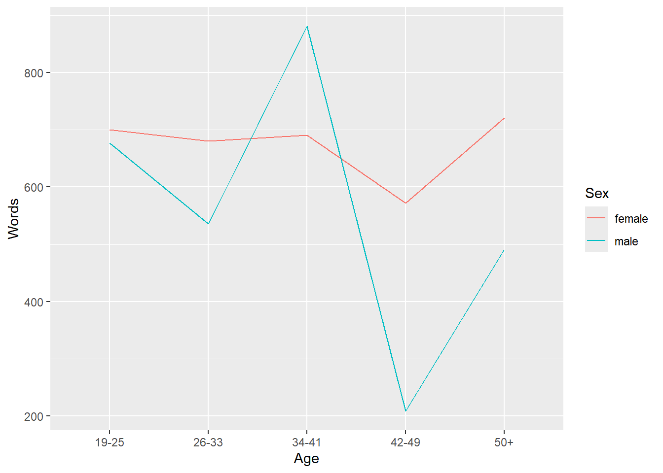

Once you have a basic plot like the one above, you can prettify the plot. For example, you can

change the width of the lines (size = 1.25)
change the y-axis limits (coord_cartesian(ylim = c(0, 1000)))
use a different theme (theme_bw() means black and white theme)
move the legend to the top
change the default colors to colors you like (*scale_color_manual …`)
change the linetype (scale_linetype_manual ...)

ggplot(plotdata, aes(x = Age, y = Words,
                     color = Sex, 
                     group = Sex, 
                     linetype = Sex)) +
  geom_line(size = 1.25) +
  coord_cartesian(ylim = c(0, 1500)) +
  theme_bw() + 
  theme(legend.position = "top") + 
  scale_color_manual(breaks = c("female", "male"),
                     values = c("gray20", "gray50")) +
  scale_linetype_manual(breaks = c("female", "male"),
                        values = c("solid", "dotted"))

An additional and very handy feature of this way of producing graphs is that you

can integrate them into pipes
can easily combine plots.

ICE_Ire %>%
  dplyr::filter(Sex != "NA",
         Age != "NA",
         is.na(Sex) == F,
         is.na(Age) == F) %>%
  dplyr::mutate(Age = factor(Age),
         Sex = factor(Sex)) %>%
  ggplot(aes(x = Age, 
             y = Word.count,
             color = Sex,
             linetype = Sex)) +
  geom_point() +
  stat_summary(fun=mean, geom="line", aes(group=Sex)) +
  coord_cartesian(ylim = c(0, 2000)) +
  theme_bw() + 
  theme(legend.position = "top") + 
  scale_color_manual(breaks = c("female", "male"),
                     values = c("indianred", "darkblue")) +
  scale_linetype_manual(breaks = c("female", "male"),
                        values = c("solid", "dotted"))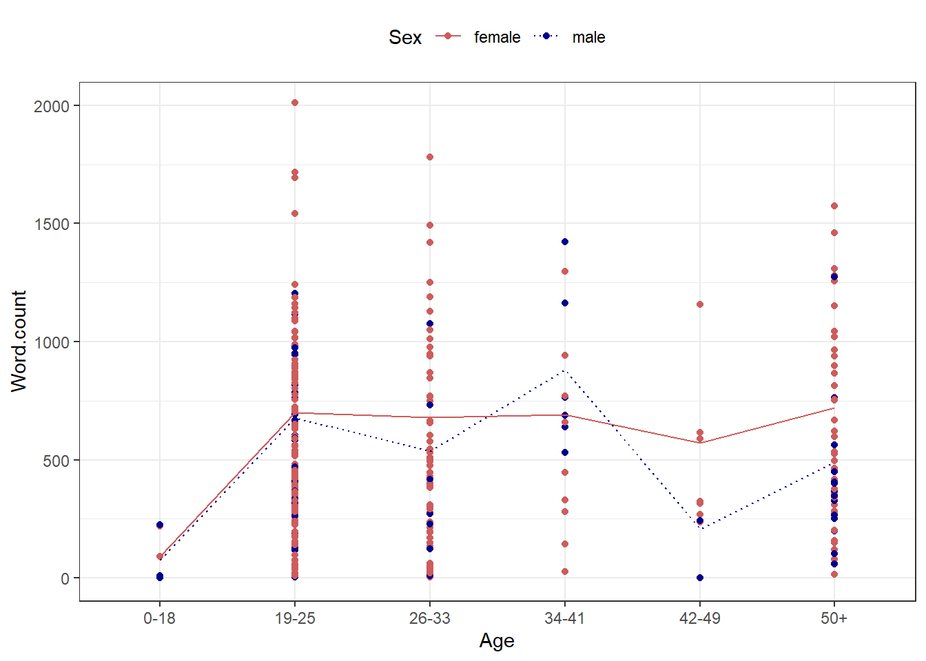

You can also create different types of graphs very easily and split them into different facets.

ICE_Ire %>%
  drop_na() %>%
  dplyr::filter(Age != "NA") %>%
  dplyr::mutate(Date = factor(Date)) %>%
  ggplot(aes(x = Age, 
             y = Word.count, 
             fill = Sex)) +
  facet_grid(vars(Date)) +
  geom_boxplot() +
  coord_cartesian(ylim = c(0, 2000)) +
  theme_bw() + 
  theme(legend.position = "top") + 
  scale_fill_manual(breaks = c("female", "male"),
                     values = c("#E69F00", "#56B4E9"))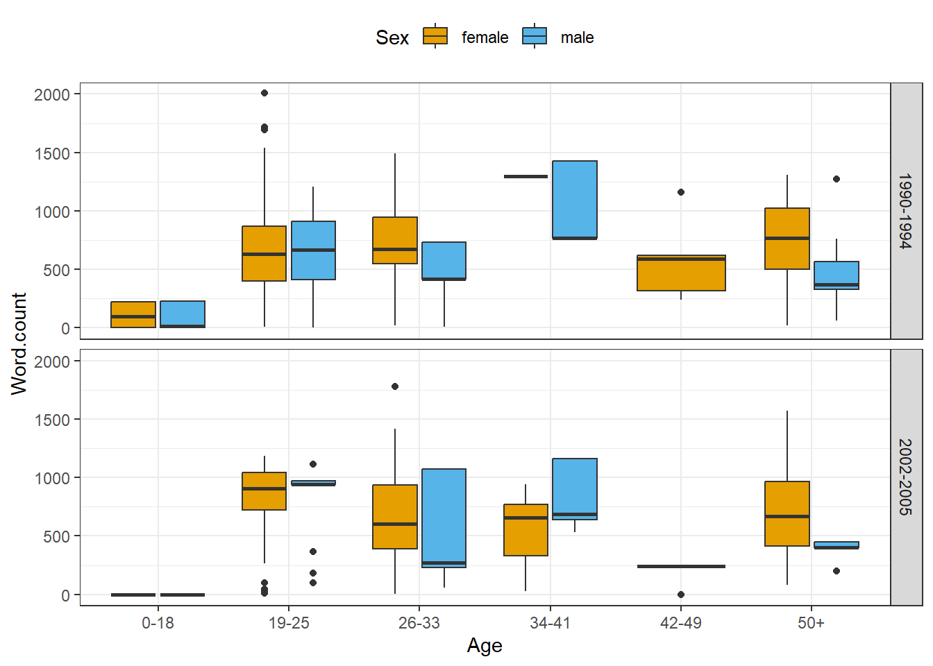

EXERCISE TIME!

Create a box plot showing the Date on the x-axis and the words uttered by speakers on the y-axis and group bySex. Answer

  ICE_Ire %>%
  drop_na() %>%
  dplyr::filter(Sex != "NA") %>%
  dplyr::mutate(Date = factor(Date)) %>%
  ggplot(aes(x = Date, 
             y = Word.count, 
             fill = Sex)) +
  geom_boxplot() +
  coord_cartesian(ylim = c(0, 2000)) +
  theme_bw() + 
  theme(legend.position = "top") + 
  scale_fill_manual(breaks = c("female", "male"),
                     values = c("#E69F00", "#56B4E9"))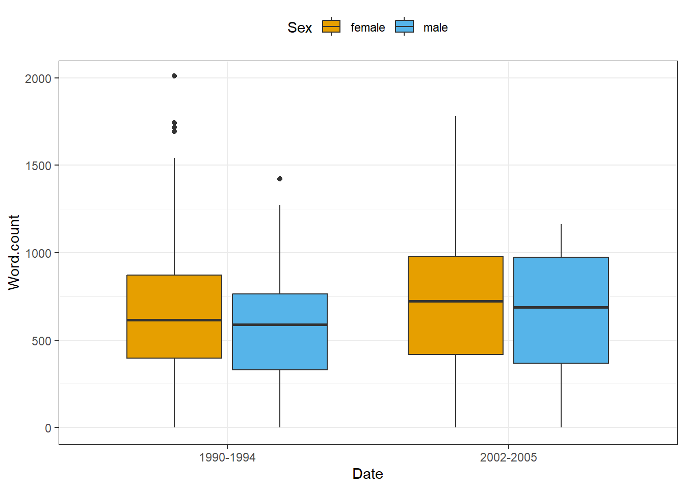

Create a scatter plot showing the Date on the x-axis and the words uttered by speakers on the y-axis and create different facets for Sex. Answer

  ICE_Ire %>%
  drop_na() %>%
  dplyr::filter(Sex != "NA",
         Date != "NA") %>%
  dplyr::mutate(Date = factor(Date),
         Sex = factor(Sex)) %>%
  ggplot(aes(Date, Word.count,
         color = Date)) +
  facet_wrap(vars(Sex), ncol = 2) +
  geom_point() +
  coord_cartesian(ylim = c(0, 2000)) +
  theme_bw() + 
  scale_color_manual(breaks = c("1990-1994", "2002-2005"),
                     values = c("#E69F00", "#56B4E9"))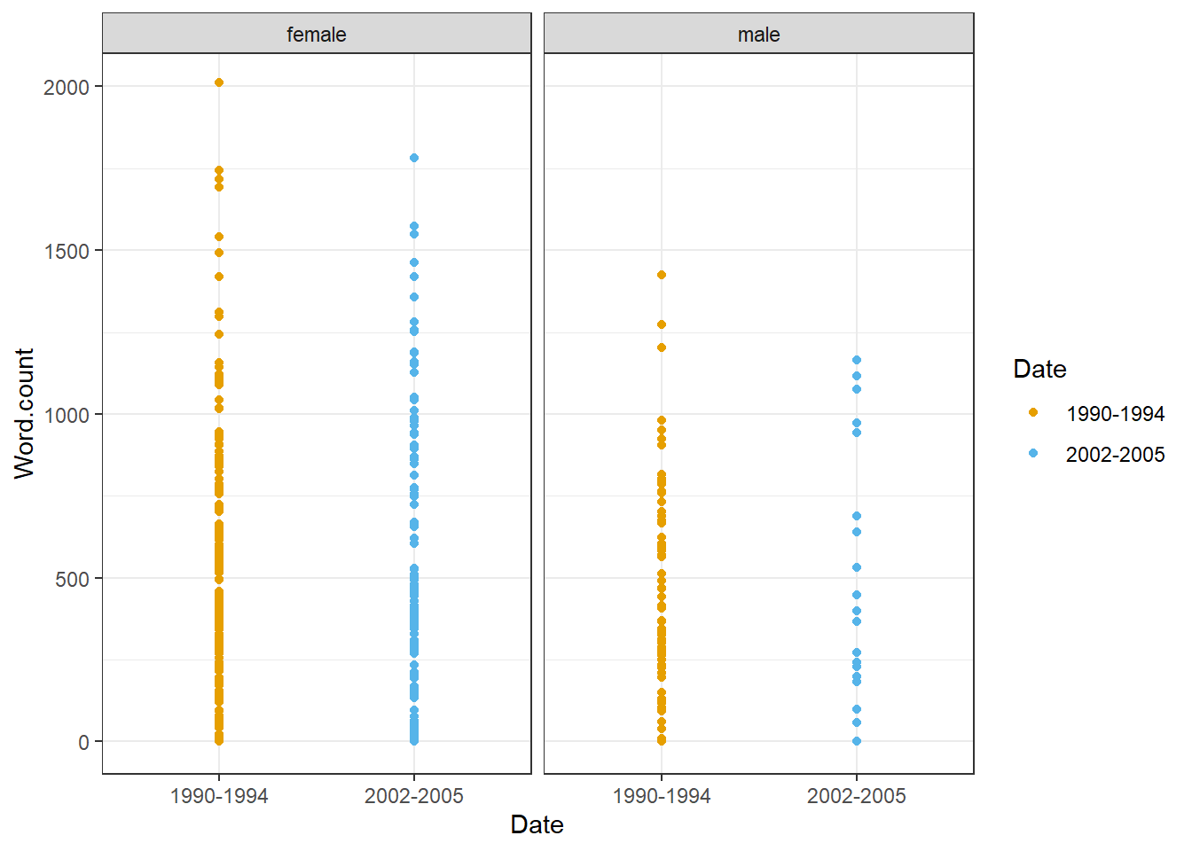

Advanced

Create a bar plot showing the number of men and women byDate.

Solution

Ending R sessions

At the end of each session, you can extract information about the session itself (e.g. which R version you used and which versions of packages). This can help others (or even your future self) to reproduce the analysis that you have done.

Going further

Here are also some additional resources that you may find helpful:

Grolemund. G., and Wickham, H., R 4 Data Science, 2017.
- Highly recommended! (especially chapters 1, 2, 4, 6, and 8)
Stat545 - Data wrangling, exploration, and analysis with R. University of British Columbia. http://stat545.com/
Swirlstats, a package that teaches you R and statistics within R: https://swirlstats.com/
DataCamp’s (free) Intro to R interactive tutorial: https://www.datacamp.com/courses/free-introduction-to-r
- DataCamp’s advanced R tutorials require a subscription. *Twitter:
- Explore RStudio Tips https://twitter.com/rstudiotips
- Explore #rstats, #rstudioconf

Citation & Session Info

Schweinberger, Martin. 2022. Getting started with R. Brisbane: The University of Queensland. url: https://ladal.edu.au/intror.html (Version 2022.11.15).

@manual{schweinberger2022intror,
  author = {Schweinberger, Martin},
  title = {Getting started with R},
  note = {https://ladal.edu.au/intror.html},
  year = {2022},
  organization = "The University of Queensland, School of Languages and Cultures},
  address = {Brisbane},
  edition = {2022.11.15}
}

sessionInfo()

## R version 4.3.2 (2023-10-31 ucrt)
## Platform: x86_64-w64-mingw32/x64 (64-bit)
## Running under: Windows 11 x64 (build 22621)
## 
## Matrix products: default
## 
## 
## locale:
## [1] LC_COLLATE=English_Australia.utf8  LC_CTYPE=English_Australia.utf8   
## [3] LC_MONETARY=English_Australia.utf8 LC_NUMERIC=C                      
## [5] LC_TIME=English_Australia.utf8    
## 
## time zone: Australia/Brisbane
## tzcode source: internal
## 
## attached base packages:
## [1] stats     graphics  grDevices utils     datasets  methods   base     
## 
## other attached packages:
##  [1] flextable_0.9.4  here_1.0.1       tokenizers_0.3.0 tm_0.7-11       
##  [5] NLP_0.2-1        readxl_1.4.3     quanteda_3.3.1   tidytext_0.4.1  
##  [9] lubridate_1.9.3  forcats_1.0.0    stringr_1.5.1    dplyr_1.1.4     
## [13] purrr_1.0.2      readr_2.1.5      tidyr_1.3.1      tibble_3.2.1    
## [17] ggplot2_3.5.0    tidyverse_2.0.0 
## 
## loaded via a namespace (and not attached):
##  [1] tidyselect_1.2.1        farver_2.1.1            fastmap_1.1.1          
##  [4] fontquiver_0.2.1        janeaustenr_1.0.0       promises_1.2.1         
##  [7] digest_0.6.34           timechange_0.3.0        mime_0.12              
## [10] lifecycle_1.0.4         gfonts_0.2.0            ellipsis_0.3.2         
## [13] magrittr_2.0.3          compiler_4.3.2          rlang_1.1.3            
## [16] sass_0.4.8              tools_4.3.2             utf8_1.2.4             
## [19] yaml_2.3.8              data.table_1.15.2       knitr_1.45             
## [22] labeling_0.4.3          askpass_1.2.0           stopwords_2.3          
## [25] curl_5.2.0              xml2_1.3.6              klippy_0.0.0.9500      
## [28] httpcode_0.3.0          withr_3.0.0             grid_4.3.2             
## [31] fansi_1.0.6             gdtools_0.3.6           xtable_1.8-4           
## [34] colorspace_2.1-0        scales_1.3.0            crul_1.4.0             
## [37] cli_3.6.2               rmarkdown_2.25          crayon_1.5.2           
## [40] ragg_1.2.7              generics_0.1.3          RcppParallel_5.1.7     
## [43] rstudioapi_0.15.0       tzdb_0.4.0              cachem_1.0.8           
## [46] assertthat_0.2.1        parallel_4.3.2          cellranger_1.1.0       
## [49] vctrs_0.6.5             Matrix_1.6-5            jsonlite_1.8.8         
## [52] slam_0.1-50             fontBitstreamVera_0.1.1 hms_1.1.3              
## [55] systemfonts_1.0.5       jquerylib_0.1.4         glue_1.7.0             
## [58] stringi_1.8.3           gtable_0.3.4            later_1.3.2            
## [61] munsell_0.5.0           pillar_1.9.0            htmltools_0.5.7        
## [64] openssl_2.1.1           R6_2.5.1                textshaping_0.3.7      
## [67] rprojroot_2.0.4         evaluate_0.23           shiny_1.8.0            
## [70] lattice_0.21-9          highr_0.10              SnowballC_0.7.1        
## [73] fontLiberation_0.1.0    httpuv_1.6.14           bslib_0.6.1            
## [76] zip_2.3.1               uuid_1.2-0              Rcpp_1.0.12            
## [79] fastmatch_1.1-4         officer_0.6.5           xfun_0.42              
## [82] pkgconfig_2.0.3

Back to LADAL home

References

Gillespie, Colin, and Robin Lovelace. 2016. Efficient r Programming: A Practical Guide to Smarter Programming. " O’Reilly Media, Inc.".

Wickham, Hadley, and Garrett Grolemund. 2016. R for Data Science: Import, Tidy, Transform, Visualize, and Model Data. " O’Reilly Media, Inc.".