Simulate spatial transcriptomic data (original) (raw)
Introduction
In this tutorial, we show how to use scDesign3 to simulate the single-cell spatial data.
Read in the reference data
The raw data is from the Seurat, which is a dataset generated with the Visium technology from 10x Genomics. We pre-select the top spatial variable genes.
example_sce <- readRDS((url("https://figshare.com/ndownloader/files/40582019")))
print(example_sce)
#> class: SingleCellExperiment
#> dim: 1000 2696
#> metadata(0):
#> assays(2): counts logcounts
#> rownames(1000): Calb2 Gng4 ... Fndc5 Gda
#> rowData names(0):
#> colnames(2696): AAACAAGTATCTCCCA-1 AAACACCAATAACTGC-1 ...
#>   TTGTTTCACATCCAGG-1 TTGTTTCCATACAACT-1
#> colData names(12): orig.ident nCount_Spatial ... spatial2 cell_type
#> reducedDimNames(0):
#> mainExpName: NULL
#> altExpNames(0):
To save time, we subset the top 10 genes.
example_sce <- example_sce[1:10, ]Simulation
Then, we can use this spatial dataset to generate new data by setting the parameter mu_formula as a smooth terms for the spatial coordinates.
set.seed(123)
example_simu <- scdesign3(
    sce = example_sce,
    assay_use = "counts",
    celltype = "cell_type",
    pseudotime = NULL,
    spatial = c("spatial1", "spatial2"),
    other_covariates = NULL,
    mu_formula = "s(spatial1, spatial2, bs = 'gp', k= 400)",
    sigma_formula = "1",
    family_use = "nb",
    n_cores = 2,
    usebam = FALSE,
    corr_formula = "1",
    copula = "gaussian",
    DT = TRUE,
    pseudo_obs = FALSE,
    return_model = FALSE,
    nonzerovar = FALSE,
    parallelization = "pbmcapply"
  )
Then, we can create the SinglecellExperiment object using the synthetic count matrix and store the logcounts to the input and synthetic SinglecellExperiment objects.
Visualization
We reformat the reference data and the synthetic data to visualize a few genes’ expressions and the spatial locations.
VISIUM_dat_test <- data.frame(t(log1p(counts(example_sce)))) %>% as_tibble() %>% dplyr::mutate(X = colData(example_sce)$spatial1, Y = colData(example_sce)$spatial2) %>% tidyr::pivot_longer(-c("X", "Y"), names_to = "Gene", values_to = "Expression") %>% dplyr::mutate(Method = "Reference")
VISIUM_dat_scDesign3 <- data.frame(t(log1p(counts(simu_sce)))) %>% as_tibble() %>% dplyr::mutate(X = colData(simu_sce)$spatial1, Y = colData(simu_sce)$spatial2) %>% tidyr::pivot_longer(-c("X", "Y"), names_to = "Gene", values_to = "Expression") %>% dplyr::mutate(Method = "scDesign3")
VISIUM_dat <- bind_rows(VISIUM_dat_test, VISIUM_dat_scDesign3) %>% dplyr::mutate(Method = factor(Method, levels = c("Reference", "scDesign3")))

VISIUM_dat %>% filter(Gene %in% rownames(example_sce)[1:5]) %>% ggplot(aes(x = X, y = Y, color = Expression)) + geom_point(size = 0.5) + scale_colour_gradientn(colors = viridis_pal(option = "magma")(10), limits=c(0, 8)) + coord_fixed(ratio = 1) + facet_grid(Method ~ Gene )+ theme_gray()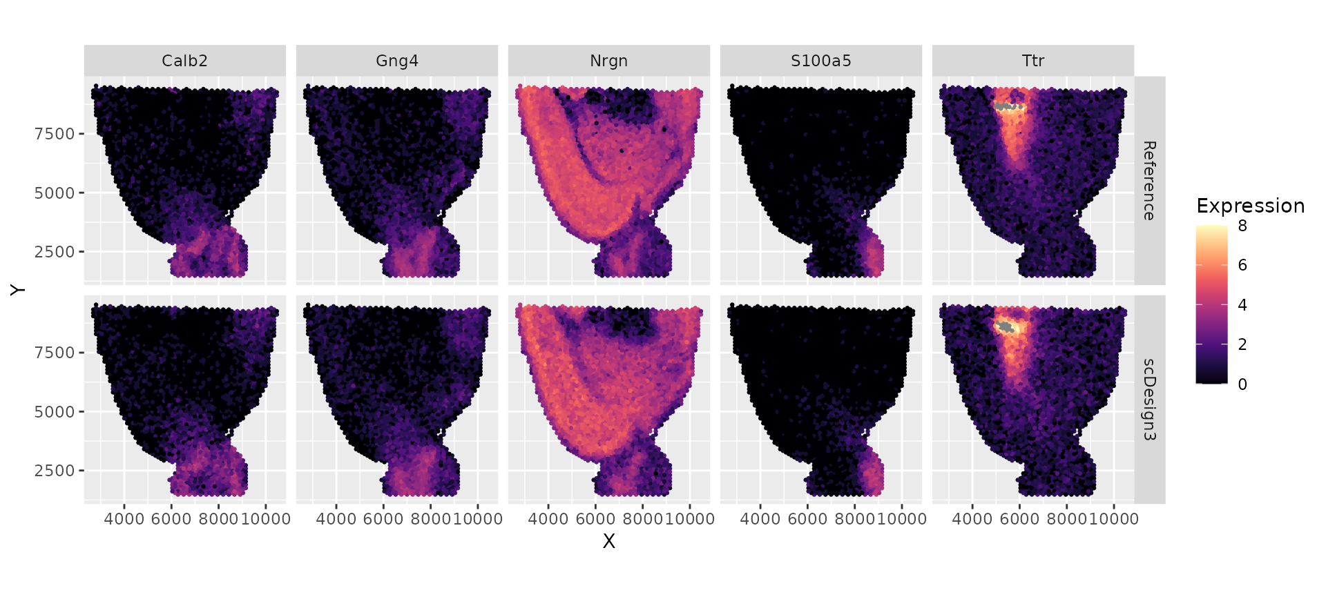
Session information
sessionInfo()
#> R version 4.3.1 (2023-06-16)
#> Platform: x86_64-pc-linux-gnu (64-bit)
#> Running under: Ubuntu 20.04.6 LTS
#>
#> Matrix products: default
#> BLAS:   /usr/lib/x86_64-linux-gnu/openblas-pthread/libblas.so.3
#> LAPACK: /usr/lib/x86_64-linux-gnu/openblas-pthread/liblapack.so.3;  LAPACK version 3.9.0
#>
#> locale:
#>  [1] LC_CTYPE=en_US.UTF-8       LC_NUMERIC=C
#>  [3] LC_TIME=en_US.UTF-8        LC_COLLATE=en_US.UTF-8
#>  [5] LC_MONETARY=en_US.UTF-8    LC_MESSAGES=en_US.UTF-8
#>  [7] LC_PAPER=en_US.UTF-8       LC_NAME=C
#>  [9] LC_ADDRESS=C               LC_TELEPHONE=C
#> [11] LC_MEASUREMENT=en_US.UTF-8 LC_IDENTIFICATION=C
#>
#> time zone: America/Los_Angeles
#> tzcode source: system (glibc)
#>
#> attached base packages:
#> [1] stats4    stats     graphics  grDevices utils     datasets  methods
#> [8] base
#>
#> other attached packages:
#>  [1] viridis_0.6.4               viridisLite_0.4.2
#>  [3] dplyr_1.1.2                 ggplot2_3.4.2
#>  [5] SingleCellExperiment_1.22.0 SummarizedExperiment_1.30.2
#>  [7] Biobase_2.60.0              GenomicRanges_1.52.0
#>  [9] GenomeInfoDb_1.36.1         IRanges_2.34.1
#> [11] S4Vectors_0.38.1            BiocGenerics_0.46.0
#> [13] MatrixGenerics_1.12.2       matrixStats_1.0.0
#> [15] scDesign3_0.99.6            BiocStyle_2.28.0
#>
#> loaded via a namespace (and not attached):
#>  [1] gtable_0.3.3            xfun_0.39               bslib_0.5.0
#>  [4] lattice_0.21-8          gamlss_5.4-12           vctrs_0.6.3
#>  [7] tools_4.3.1             bitops_1.0-7            generics_0.1.3
#> [10] parallel_4.3.1          tibble_3.2.1            fansi_1.0.4
#> [13] highr_0.10              pkgconfig_2.0.3         Matrix_1.6-0
#> [16] desc_1.4.2              lifecycle_1.0.3         GenomeInfoDbData_1.2.10
#> [19] farver_2.1.1            compiler_4.3.1          stringr_1.5.0
#> [22] textshaping_0.3.6       munsell_0.5.0           htmltools_0.5.5
#> [25] sass_0.4.7              RCurl_1.98-1.12         yaml_2.3.7
#> [28] tidyr_1.3.0             crayon_1.5.2            pillar_1.9.0
#> [31] pkgdown_2.0.7           jquerylib_0.1.4         MASS_7.3-60
#> [34] DelayedArray_0.26.6     cachem_1.0.8            mclust_6.0.0
#> [37] nlme_3.1-162            tidyselect_1.2.0        digest_0.6.33
#> [40] mvtnorm_1.2-2           stringi_1.7.12          purrr_1.0.1
#> [43] bookdown_0.34           labeling_0.4.2          splines_4.3.1
#> [46] gamlss.dist_6.0-5       rprojroot_2.0.3         fastmap_1.1.1
#> [49] grid_4.3.1              gamlss.data_6.0-2       colorspace_2.1-0
#> [52] cli_3.6.1               magrittr_2.0.3          S4Arrays_1.0.4
#> [55] survival_3.5-5          utf8_1.2.3              withr_2.5.0
#> [58] scales_1.2.1            XVector_0.40.0          rmarkdown_2.23
#> [61] gridExtra_2.3           ragg_1.2.5              memoise_2.0.1
#> [64] evaluate_0.21           knitr_1.43              mgcv_1.9-0
#> [67] rlang_1.1.1             glue_1.6.2              BiocManager_1.30.21.1
#> [70] jsonlite_1.8.7          R6_2.5.1                zlibbioc_1.46.0
#> [73] systemfonts_1.0.4       fs_1.6.3