Overview of the tidySingleCellExperiment package (original) (raw)
Introduction
tidySingleCellExperiment provides a bridge between Bioconductor single-cell packages (Amezquita et al. 2019) and the tidyverse (Wickham et al. 2019). It enables viewing the Bioconductor _SingleCellExperimentobject as a tidyverse tibble, and providesSingleCellExperiment-compatible dplyr, tidyr, ggplot2 andplotly_functions (see Table @ref(tab:table)). This allows users to get the best of both Bioconductor and tidyverse worlds.
(#tab:table) Available tidySingleCellExperimentfunctions and utilities.
| All functions compatible withSingleCellExperiments | After all, a tidySingleCellExperiment is aSingleCellExperiment, just better! |
|---|---|
| tidyverse | |
| dplyr | All tibble-compatible functions (e.g.,select()) |
| tidyr | All tibble-compatible functions (e.g.,pivot_longer()) |
| ggplot2 | Plotting with ggplot() |
| plotly | Plotting with plot_ly() |
| Utilities | |
| as_tibble() | Convert cell-wise information to a tbl_df |
| join_features() | Add feature-wise information; returns atbl_df |
| aggregate_cells() | Aggregate feature abundances as pseudobulks; returns aSummarizedExperiment |
Installation
Load libraries used in this vignette.
## Error in get(paste0(generic, ".", class), envir = get_method_env()) :
##   object 'type_sum.accel' not found
Data representation of tidySingleCellExperiment
This is a SingleCellExperiment object but it is evaluated as a tibble. So it is compatible both withSingleCellExperiment and tidyverse.
data(pbmc_small, package="tidySingleCellExperiment")
pbmc_small_tidy <- pbmc_small
It looks like a tibble…
## # A SingleCellExperiment-tibble abstraction: 80 × 17
## # Features=230 | Cells=80 | Assays=counts, logcounts
##    .cell orig.ident nCount_RNA nFeature_RNA RNA_snn_res.0.8 letter.idents groups
##    <chr> <fct>           <dbl>        <int> <fct>           <fct>         <chr>
##  1 ATGC… SeuratPro…         70           47 0               A             g2
##  2 CATG… SeuratPro…         85           52 0               A             g1
##  3 GAAC… SeuratPro…         87           50 1               B             g2
##  4 TGAC… SeuratPro…        127           56 0               A             g2
##  5 AGTC… SeuratPro…        173           53 0               A             g2
##  6 TCTG… SeuratPro…         70           48 0               A             g1
##  7 TGGT… SeuratPro…         64           36 0               A             g1
##  8 GCAG… SeuratPro…         72           45 0               A             g1
##  9 GATA… SeuratPro…         52           36 0               A             g1
## 10 AATG… SeuratPro…        100           41 0               A             g1
## # ℹ 70 more rows
## # ℹ 10 more variables: RNA_snn_res.1 <fct>, file <chr>, ident <fct>,
## #   PC_1 <dbl>, PC_2 <dbl>, PC_3 <dbl>, PC_4 <dbl>, PC_5 <dbl>, tSNE_1 <dbl>,
## #   tSNE_2 <dbl>
…but it is a SingleCellExperiment after all!
counts(pbmc_small_tidy)[1:5, 1:4]## 5 x 4 sparse Matrix of class "dgCMatrix"
## ATGCCAGAACGACT CATGGCCTGTGCAT GAACCTGATGAACC TGACTGGATTCTCA
## MS4A1 . . . .
## CD79B 1 . . .
## CD79A . . . .
## HLA-DRA . 1 . .
## TCL1A . . . .The SingleCellExperiment object’s tibble visualisation can be turned off, or back on at any time.
# Turn off the tibble visualisation
options("restore_SingleCellExperiment_show" = TRUE)
pbmc_small_tidy
## class: SingleCellExperiment
## dim: 230 80
## metadata(0):
## assays(2): counts logcounts
## rownames(230): MS4A1 CD79B ... SPON2 S100B
## rowData names(5): vst.mean vst.variance vst.variance.expected
## vst.variance.standardized vst.variable
## colnames(80): ATGCCAGAACGACT CATGGCCTGTGCAT ... GGAACACTTCAGAC
## CTTGATTGATCTTC
## colData names(9): orig.ident nCount_RNA ... file ident# Turn on the tibble visualisation
options("restore_SingleCellExperiment_show" = FALSE)Annotation polishing
We may have a column that contains the directory each run was taken from, such as the “file” column in pbmc_small_tidy.
pbmc_small_tidy$file[1:5]## [1] "../data/sample2/outs/filtered_feature_bc_matrix/"
## [2] "../data/sample1/outs/filtered_feature_bc_matrix/"
## [3] "../data/sample2/outs/filtered_feature_bc_matrix/"
## [4] "../data/sample2/outs/filtered_feature_bc_matrix/"
## [5] "../data/sample2/outs/filtered_feature_bc_matrix/"We may want to extract the run/sample name out of it into a separate column. The tidyverse function [extract()](../reference/extract.html) can be used to convert a character column into multiple columns using regular expression groups.
# Create sample column
pbmc_small_polished <-
    pbmc_small_tidy %>%
    extract(file, "sample", "../data/([a-z0-9]+)/outs.+", remove=FALSE)

# Reorder to have sample column up front
pbmc_small_polished %>%
    select(sample, everything())
## # A SingleCellExperiment-tibble abstraction: 80 × 18
## # Features=230 | Cells=80 | Assays=counts, logcounts
## .cell sample orig.ident nCount_RNA nFeature_RNA RNA_snn_res.0.8 letter.idents
## <chr> <chr> <fct> <dbl> <int> <fct> <fct>
## 1 ATGC… sampl… SeuratPro… 70 47 0 A
## 2 CATG… sampl… SeuratPro… 85 52 0 A
## 3 GAAC… sampl… SeuratPro… 87 50 1 B
## 4 TGAC… sampl… SeuratPro… 127 56 0 A
## 5 AGTC… sampl… SeuratPro… 173 53 0 A
## 6 TCTG… sampl… SeuratPro… 70 48 0 A
## 7 TGGT… sampl… SeuratPro… 64 36 0 A
## 8 GCAG… sampl… SeuratPro… 72 45 0 A
## 9 GATA… sampl… SeuratPro… 52 36 0 A
## 10 AATG… sampl… SeuratPro… 100 41 0 A
## # ℹ 70 more rows
## # ℹ 11 more variables: groups <chr>, RNA_snn_res.1 <fct>, file <chr>,
## # ident <fct>, PC_1 <dbl>, PC_2 <dbl>, PC_3 <dbl>, PC_4 <dbl>, PC_5 <dbl>,
## # tSNE_1 <dbl>, tSNE_2 <dbl>Preliminary plots
Set colours and theme for plots.
# Use colourblind-friendly colours
friendly_cols <- dittoSeq::dittoColors()
# Set theme
custom_theme <- list(
scale_fill_manual(values=friendly_cols),
scale_color_manual(values=friendly_cols),
theme_bw() + theme(
aspect.ratio=1,
legend.position="bottom",
axis.line=element_line(),
text=element_text(size=12),
panel.border=element_blank(),
strip.background=element_blank(),
panel.grid.major=element_line(linewidth=0.2),
panel.grid.minor=element_line(linewidth=0.1),
axis.title.x=element_text(margin=margin(t=10, r=10, b=10, l=10)),
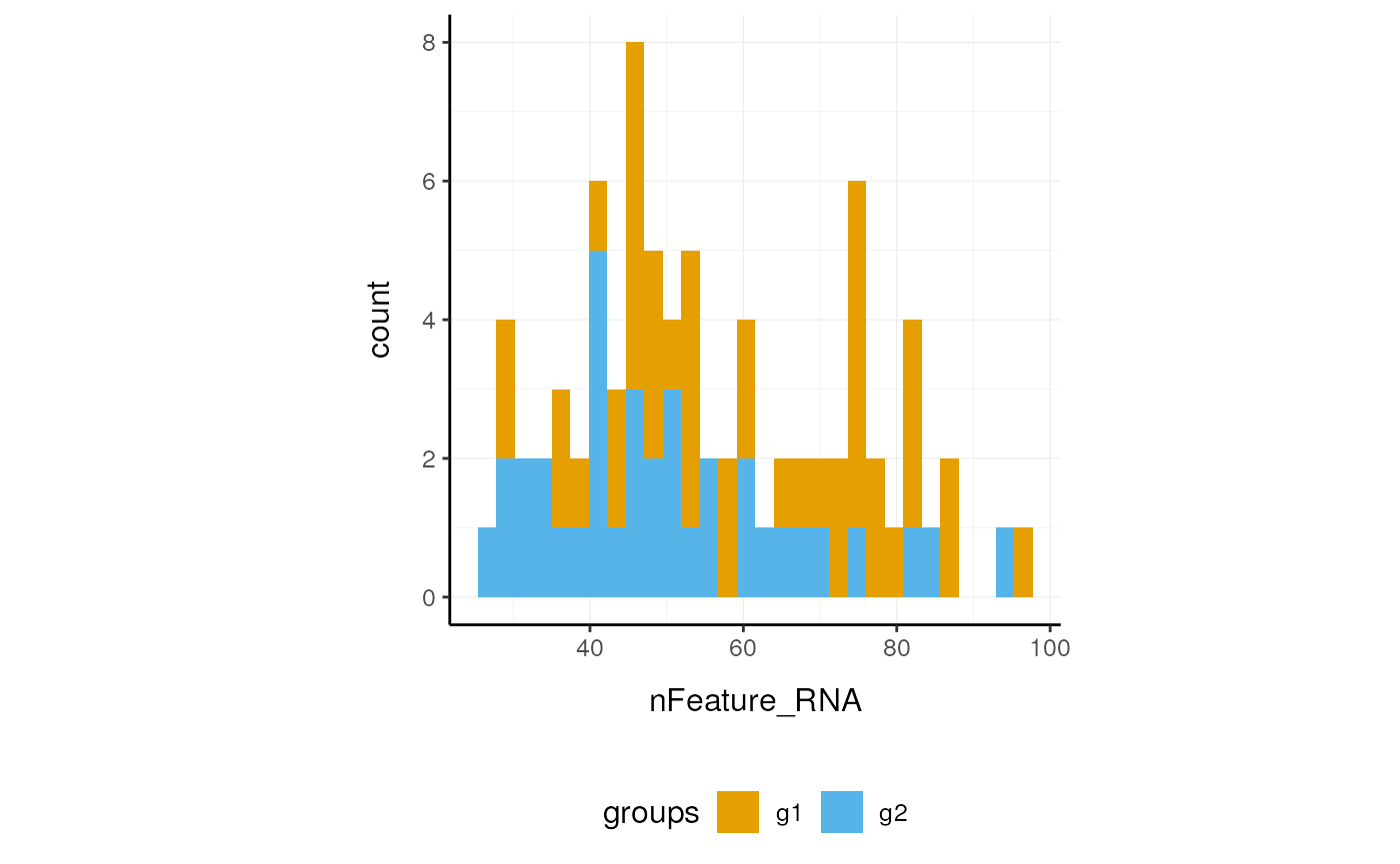
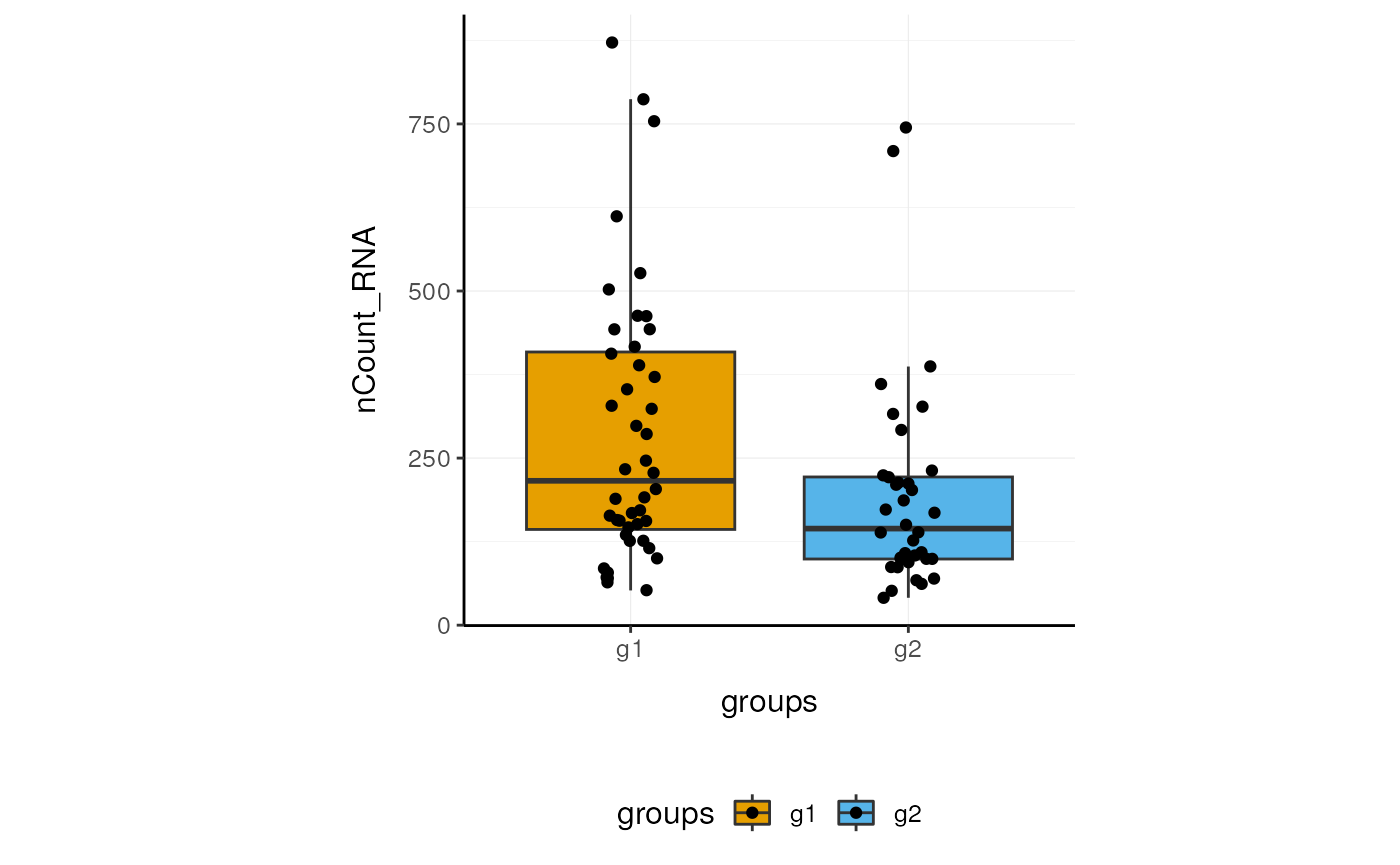
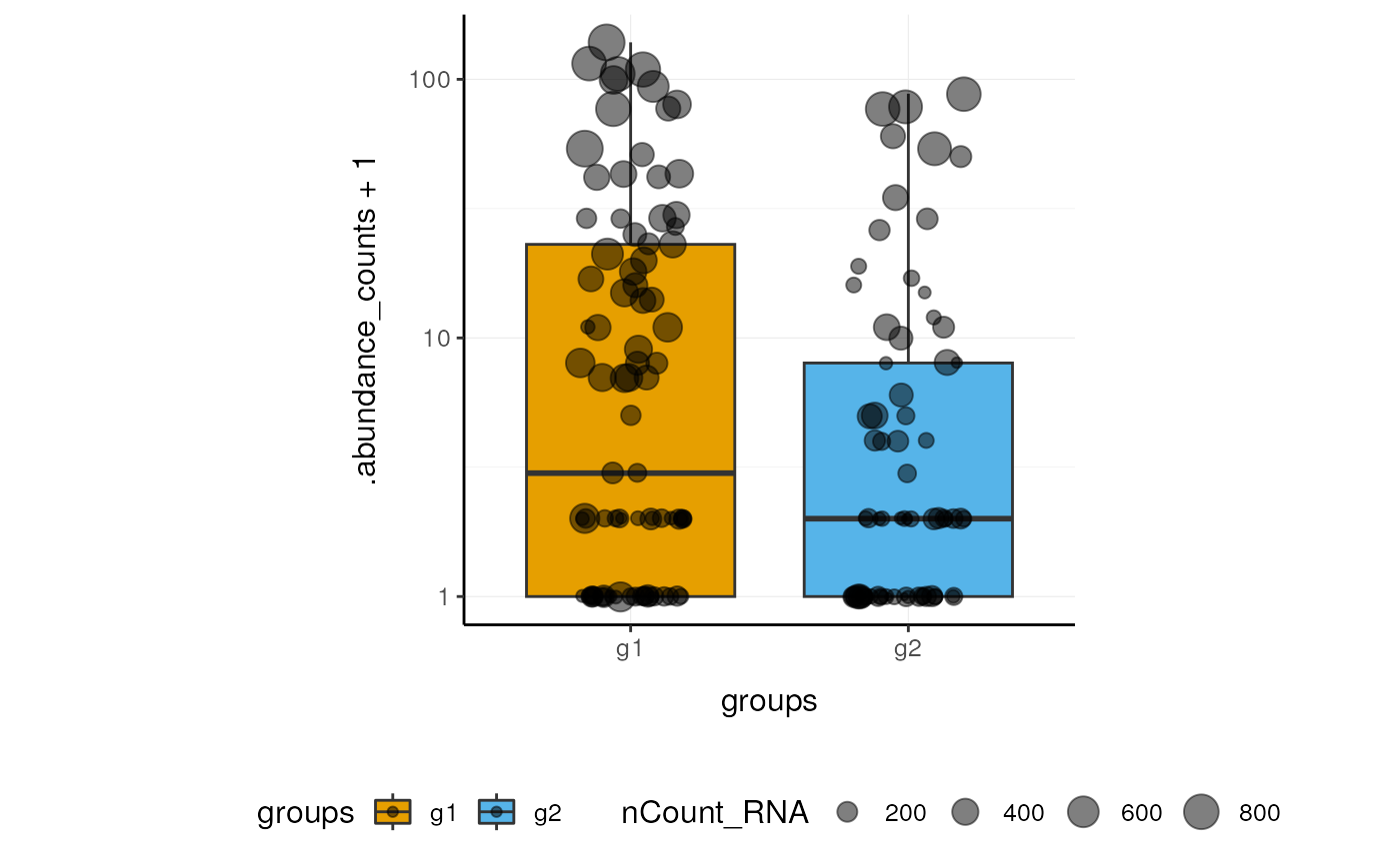
axis.title.y=element_text(margin=margin(t=10, r=10, b=10, l=10))))We can treat pbmc_small_polished as atibble for plotting.
Here we plot number of features per cell.
Here we plot total features per cell.
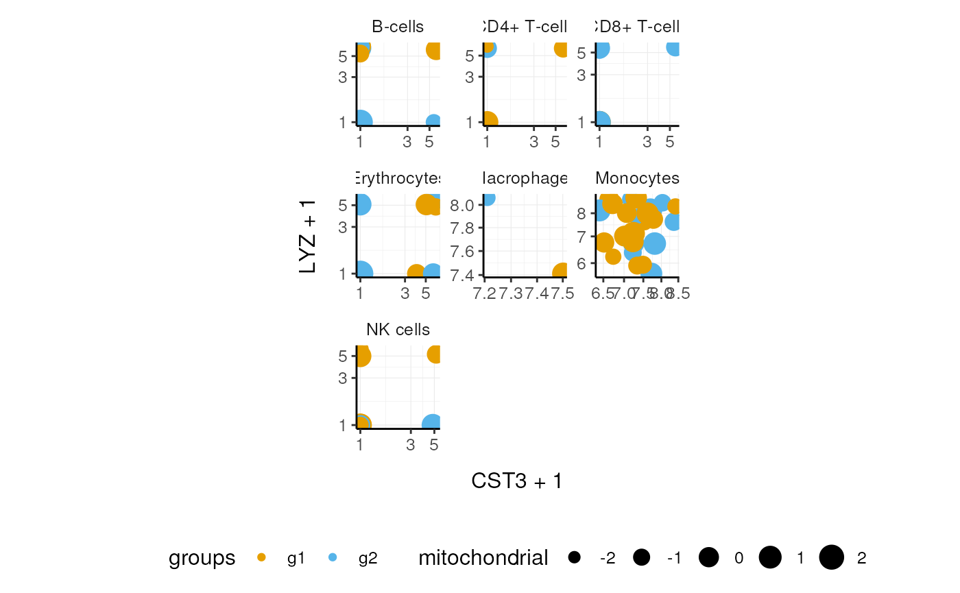
Here we plot abundance of two features for each group.
Preprocessing
We can also treat pbmc_small_polished as aSingleCellExperiment object and proceed with data processing with Bioconductor packages, such as scran (Lun, Bach, and Marioni 2016) and scater (McCarthy et al. 2017).
# Identify variable genes with scran
variable_genes <-
    pbmc_small_polished %>%
    modelGeneVar() %>%
    getTopHVGs(prop=0.1)

# Perform PCA with scater
pbmc_small_pca <-
    pbmc_small_polished %>%
    runPCA(subset_row=variable_genes)

pbmc_small_pca
## # A SingleCellExperiment-tibble abstraction: 80 × 18
## # Features=230 | Cells=80 | Assays=counts, logcounts
## .cell orig.ident nCount_RNA nFeature_RNA RNA_snn_res.0.8 letter.idents groups
## <chr> <fct> <dbl> <int> <fct> <fct> <chr>
## 1 ATGC… SeuratPro… 70 47 0 A g2
## 2 CATG… SeuratPro… 85 52 0 A g1
## 3 GAAC… SeuratPro… 87 50 1 B g2
## 4 TGAC… SeuratPro… 127 56 0 A g2
## 5 AGTC… SeuratPro… 173 53 0 A g2
## 6 TCTG… SeuratPro… 70 48 0 A g1
## 7 TGGT… SeuratPro… 64 36 0 A g1
## 8 GCAG… SeuratPro… 72 45 0 A g1
## 9 GATA… SeuratPro… 52 36 0 A g1
## 10 AATG… SeuratPro… 100 41 0 A g1
## # ℹ 70 more rows
## # ℹ 11 more variables: RNA_snn_res.1 <fct>, file <chr>, sample <chr>,
## # ident <fct>, PC1 <dbl>, PC2 <dbl>, PC3 <dbl>, PC4 <dbl>, PC5 <dbl>,
## # tSNE_1 <dbl>, tSNE_2 <dbl>If a _tidyverse_-compatible package is not included in thetidySingleCellExperiment collection, we can use[as_tibble()](../reference/as%5Ftibble.html) to permanently convert atidySingleCellExperiment into a tibble.
# Create pairs plot with 'GGally'
pbmc_small_pca %>%
    as_tibble() %>%
    select(contains("PC"), everything()) %>%
    GGally::ggpairs(columns=1:5, aes(colour=groups)) +
    custom_theme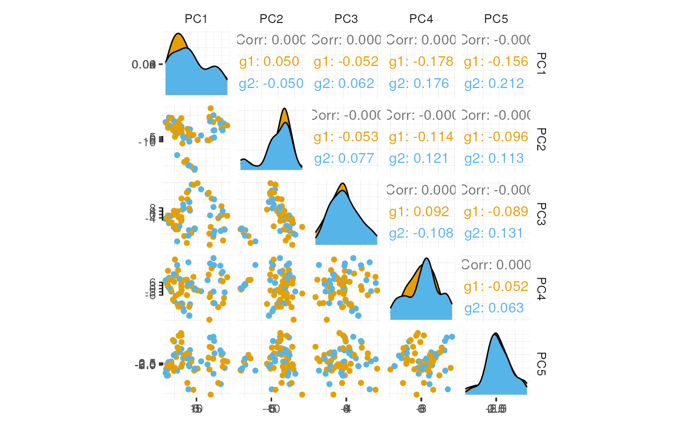
Clustering
We can proceed with cluster identification with scran.
## # A SingleCellExperiment-tibble abstraction: 80 × 19
## # Features=230 | Cells=80 | Assays=counts, logcounts
##    .cell  label orig.ident nCount_RNA nFeature_RNA RNA_snn_res.0.8 letter.idents
##    <chr>  <fct> <fct>           <dbl>        <int> <fct>           <fct>
##  1 ATGCC… 2     SeuratPro…         70           47 0               A
##  2 CATGG… 2     SeuratPro…         85           52 0               A
##  3 GAACC… 2     SeuratPro…         87           50 1               B
##  4 TGACT… 1     SeuratPro…        127           56 0               A
##  5 AGTCA… 2     SeuratPro…        173           53 0               A
##  6 TCTGA… 2     SeuratPro…         70           48 0               A
##  7 TGGTA… 1     SeuratPro…         64           36 0               A
##  8 GCAGC… 2     SeuratPro…         72           45 0               A
##  9 GATAT… 2     SeuratPro…         52           36 0               A
## 10 AATGT… 2     SeuratPro…        100           41 0               A
## # ℹ 70 more rows
## # ℹ 12 more variables: groups <chr>, RNA_snn_res.1 <fct>, file <chr>,
## #   sample <chr>, ident <fct>, PC1 <dbl>, PC2 <dbl>, PC3 <dbl>, PC4 <dbl>,
## #   PC5 <dbl>, tSNE_1 <dbl>, tSNE_2 <dbl>
And interrogate the output as if it was a regulartibble.
# Count number of cells for each cluster per group
pbmc_small_cluster %>%
    count(groups, label)
## # A tibble: 8 × 3
## groups label n
## <chr> <fct> <int>
## 1 g1 1 12
## 2 g1 2 14
## 3 g1 3 14
## 4 g1 4 4
## 5 g2 1 10
## 6 g2 2 11
## 7 g2 3 10
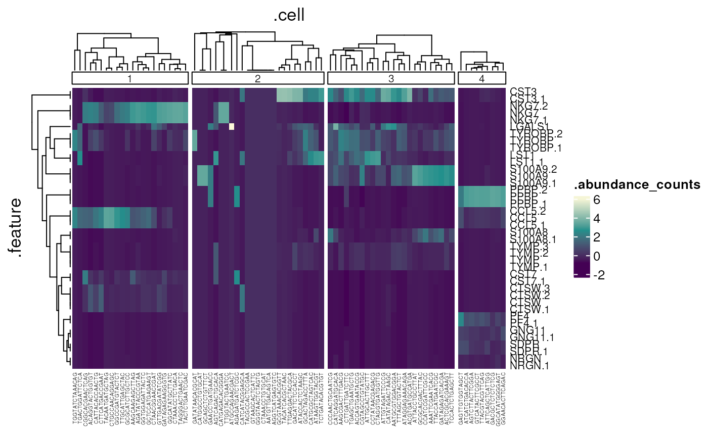
## 8 g2 4 5We can identify and visualise cluster markers combiningSingleCellExperiment, tidyverse functions and_tidyHeatmap_ (Mangiola and Papenfuss 2020).
Reduce dimensions
We can calculate the first 3 UMAP dimensions using scater.
pbmc_small_UMAP <-
    pbmc_small_cluster %>%
    runUMAP(ncomponents=3)
And we can plot the result in 3D using plotly.
pbmc_small_UMAP %>%
    plot_ly(
        x=~`UMAP1`,
        y=~`UMAP2`,
        z=~`UMAP3`,
        color=~label,
        colors=friendly_cols[1:4])
plotly screenshot
Cell type prediction
We can infer cell type identities using SingleR (Aran et al. 2019) and manipulate the output using tidyverse.
# Join UMAP and cell type info
data(cell_type_df)
pbmc_small_cell_type <-
    pbmc_small_UMAP %>%
    left_join(cell_type_df, by="cell")

# Reorder columns
pbmc_small_cell_type %>%
    select(cell, first.labels, everything())
## # A SingleCellExperiment-tibble abstraction: 80 × 23
## # Features=230 | Cells=80 | Assays=counts, logcounts
## cell first.labels orig.ident nCount_RNA nFeature_RNA RNA_snn_res.0.8
## <chr> <chr> <fct> <dbl> <int> <fct>
## 1 ATGCCAGAACGA… CD4+ T-cells SeuratPro… 70 47 0
## 2 CATGGCCTGTGC… CD8+ T-cells SeuratPro… 85 52 0
## 3 GAACCTGATGAA… CD8+ T-cells SeuratPro… 87 50 1
## 4 TGACTGGATTCT… CD4+ T-cells SeuratPro… 127 56 0
## 5 AGTCAGACTGCA… CD4+ T-cells SeuratPro… 173 53 0
## 6 TCTGATACACGT… CD4+ T-cells SeuratPro… 70 48 0
## 7 TGGTATCTAAAC… CD4+ T-cells SeuratPro… 64 36 0
## 8 GCAGCTCTGTTT… CD4+ T-cells SeuratPro… 72 45 0
## 9 GATATAACACGC… CD4+ T-cells SeuratPro… 52 36 0
## 10 AATGTTGACAGT… CD4+ T-cells SeuratPro… 100 41 0
## # ℹ 70 more rows
## # ℹ 17 more variables: letter.idents <fct>, groups <chr>, RNA_snn_res.1 <fct>,
## # file <chr>, sample <chr>, ident <fct>, label <fct>, PC1 <dbl>, PC2 <dbl>,
## # PC3 <dbl>, PC4 <dbl>, PC5 <dbl>, tSNE_1 <dbl>, tSNE_2 <dbl>, UMAP1 <dbl>,
## # UMAP2 <dbl>, UMAP3 <dbl>We can easily summarise the results. For example, we can see how cell type classification overlaps with cluster classification.
# Count number of cells for each cell type per cluster
pbmc_small_cell_type %>%
    count(label, first.labels)
## # A tibble: 11 × 3
## label first.labels n
## <fct> <chr> <int>
## 1 1 CD4+ T-cells 2
## 2 1 CD8+ T-cells 8
## 3 1 NK cells 12
## 4 2 B-cells 10
## 5 2 CD4+ T-cells 6
## 6 2 CD8+ T-cells 2
## 7 2 Macrophages 1
## 8 2 Monocytes 6
## 9 3 Macrophages 1
## 10 3 Monocytes 23
## 11 4 Erythrocytes 9We can easily reshape the data for building information-rich faceted plots.
pbmc_small_cell_type %>%
    # Reshape and add classifier column
    pivot_longer(
        cols=c(label, first.labels),
        names_to="classifier", values_to="label") %>%
    # UMAP plots for cell type and cluster
    ggplot(aes(UMAP1, UMAP2, color=label)) +
    facet_wrap(~classifier) +
    geom_point() +
    custom_theme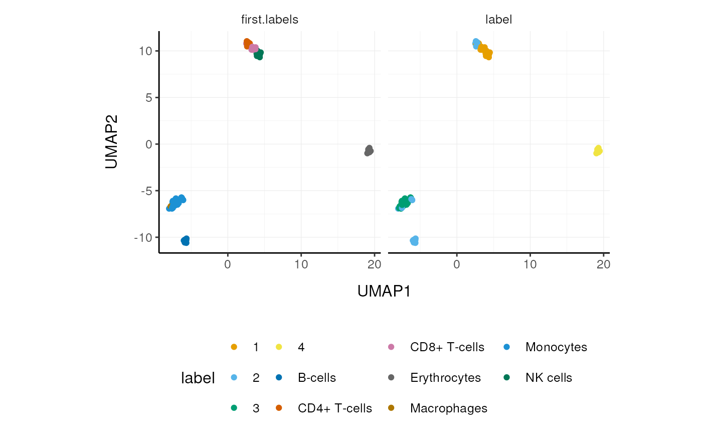
We can easily plot gene correlation per cell category, adding multi-layer annotations.
Nested analyses
A powerful tool we can use with tidySingleCellExperimentis _tidyverse_’s [nest()](../reference/nest.html). We can easily perform independent analyses on subsets of the dataset. First, we classify cell types into lymphoid and myeloid, and then [nest()](../reference/nest.html) based on the new classification.
pbmc_small_nested <-
    pbmc_small_cell_type %>%
    filter(first.labels != "Erythrocytes") %>%
    mutate(cell_class=if_else(
        first.labels %in% c("Macrophages", "Monocytes"),
        true="myeloid", false="lymphoid")) %>%
    nest(data=-cell_class)

pbmc_small_nested
## # A tibble: 2 × 2
## cell_class data
## <chr> <list>
## 1 lymphoid <SnglCllE[,40]>
## 2 myeloid <SnglCllE[,31]>Now we can independently for the lymphoid and myeloid subsets (i) find variable features, (ii) reduce dimensions, and (iii) cluster using both tidyverse and SingleCellExperiment seamlessly.
## # A tibble: 2 × 2
##   cell_class data
##   <chr>      <list>
## 1 lymphoid   <SnglCllE[,40]>
## 2 myeloid <SnglCllE[,31]>We can then [unnest()](../reference/unnest.html) and plot the new classification.
pbmc_small_nested_reanalysed %>%
    # Convert to 'tibble', else 'SingleCellExperiment'
    # drops reduced dimensions when unifying data sets.
    mutate(data=map(data, ~as_tibble(.x))) %>%
    unnest(data) %>%
    # Define unique clusters
    unite("cluster", c(cell_class, label), remove=FALSE) %>%
    # Plotting
    ggplot(aes(UMAP1, UMAP2, color=cluster)) +
    facet_wrap(~cell_class) +
    geom_point() +
    custom_theme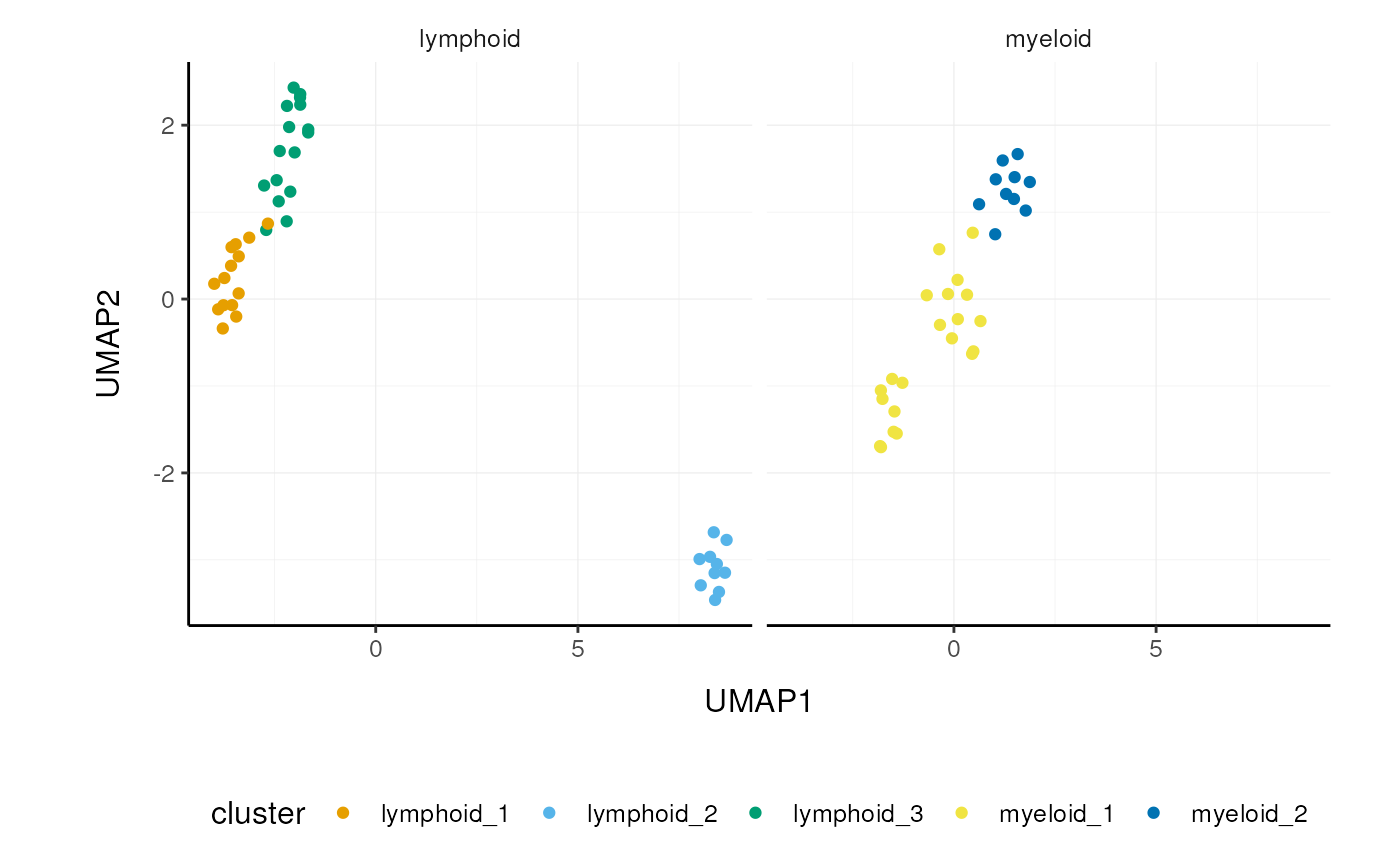
We can perform a large number of functional analyses on data subsets. For example, we can identify intra-sample cell-cell interactions usingSingleCellSignalR (Cabello-Aguilar et al. 2020), and then compare whether interactions are stronger or weaker across conditions. The code below demonstrates how this analysis could be performed. It won’t work with this small example dataset as we have just two samples (one for each condition). But some example output is shown below and you can imagine how you can use tidyverse on the output to perform t-tests and visualisation.
If the dataset was not so small, and interactions could be identified, you would see something like below.
data(pbmc_small_nested_interactions)
pbmc_small_nested_interactions
## # A tibble: 100 × 9
## sample ligand receptor ligand.name receptor.name origin destination
## <chr> <chr> <chr> <chr> <chr> <chr> <chr>
## 1 sample1 cluster 1.PTMA cluster… PTMA VIPR1 clust… cluster 2
## 2 sample1 cluster 1.B2M cluster… B2M KLRD1 clust… cluster 2
## 3 sample1 cluster 1.IL16 cluster… IL16 CD4 clust… cluster 2
## 4 sample1 cluster 1.HLA-B cluster… HLA-B KLRD1 clust… cluster 2
## 5 sample1 cluster 1.CALM1 cluster… CALM1 VIPR1 clust… cluster 2
## 6 sample1 cluster 1.HLA-E cluster… HLA-E KLRD1 clust… cluster 2
## 7 sample1 cluster 1.GNAS cluster… GNAS VIPR1 clust… cluster 2
## 8 sample1 cluster 1.B2M cluster… B2M HFE clust… cluster 2
## 9 sample1 cluster 1.PTMA cluster… PTMA VIPR1 clust… cluster 3
## 10 sample1 cluster 1.CALM1 cluster… CALM1 VIPR1 clust… cluster 3
## # ℹ 90 more rows
## # ℹ 2 more variables: interaction.type <chr>, LRscore <dbl>Aggregating cells
Sometimes, it is necessary to aggregate the gene-transcript abundance from a group of cells into a single value. For example, when comparing groups of cells across different samples with fixed-effect models.
In tidySingleCellExperiment, cell aggregation can be achieved using [aggregate_cells()](../reference/aggregate%5Fcells.html), which will return an object of class SummarizedExperiment.
## class: SummarizedExperiment
## dim: 230 2
## metadata(0):
## assays(1): counts
## rownames(230): ACAP1 ACRBP ... ZNF330 ZNF76
## rowData names(5): vst.mean vst.variance vst.variance.expected
##   vst.variance.standardized vst.variable
## colnames(2): g1 g2
## colData names(4): .aggregated_cells groups orig.ident file
Session Info
## R Under development (unstable) (2024-12-17 r87446)
## Platform: x86_64-pc-linux-gnu
## Running under: Ubuntu 24.04.1 LTS
##
## Matrix products: default
## BLAS:   /usr/lib/x86_64-linux-gnu/openblas-pthread/libblas.so.3
## LAPACK: /usr/lib/x86_64-linux-gnu/openblas-pthread/libopenblasp-r0.3.26.so;  LAPACK version 3.12.0
##
## locale:
##  [1] LC_CTYPE=en_US.UTF-8       LC_NUMERIC=C
##  [3] LC_TIME=en_US.UTF-8        LC_COLLATE=en_US.UTF-8
##  [5] LC_MONETARY=en_US.UTF-8    LC_MESSAGES=en_US.UTF-8
##  [7] LC_PAPER=en_US.UTF-8       LC_NAME=C
##  [9] LC_ADDRESS=C               LC_TELEPHONE=C
## [11] LC_MEASUREMENT=en_US.UTF-8 LC_IDENTIFICATION=C
##
## time zone: UTC
## tzcode source: system (glibc)
##
## attached base packages:
## [1] stats4    stats     graphics  grDevices utils     datasets  methods
## [8] base
##
## other attached packages:
##  [1] dittoSeq_1.19.0                 Matrix_1.7-1
##  [3] ttservice_0.4.1                 tidyr_1.3.1
##  [5] dplyr_1.1.4                     tidySingleCellExperiment_1.15.6
##  [7] tidyHeatmap_1.8.1               GGally_2.2.1
##  [9] purrr_1.0.2                     SingleCellSignalR_1.19.0
## [11] SingleR_2.9.3                   celldex_1.17.0
## [13] igraph_2.1.2                    scater_1.35.0
## [15] ggplot2_3.5.1                   scran_1.35.0
## [17] scuttle_1.17.0                  SingleCellExperiment_1.29.1
## [19] SummarizedExperiment_1.37.0     Biobase_2.67.0
## [21] GenomicRanges_1.59.1            GenomeInfoDb_1.43.2
## [23] IRanges_2.41.2                  S4Vectors_0.45.2
## [25] BiocGenerics_0.53.3             generics_0.1.3
## [27] MatrixGenerics_1.19.0           matrixStats_1.4.1
## [29] knitr_1.49                      BiocStyle_2.35.0
##
## loaded via a namespace (and not attached):
##   [1] splines_4.5.0             bitops_1.0-9
##   [3] filelock_1.0.3            tibble_3.2.1
##   [5] lifecycle_1.0.4           httr2_1.0.7
##   [7] doParallel_1.0.17         edgeR_4.5.1
##   [9] lattice_0.22-6            MASS_7.3-61
##  [11] alabaster.base_1.7.2      dendextend_1.19.0
##  [13] magrittr_2.0.3            plotly_4.10.4
##  [15] limma_3.63.2              sass_0.4.9
##  [17] rmarkdown_2.29            jquerylib_0.1.4
##  [19] yaml_2.3.10               metapod_1.15.0
##  [21] cowplot_1.1.3             DBI_1.2.3
##  [23] RColorBrewer_1.1-3        abind_1.4-8
##  [25] zlibbioc_1.53.0           Rtsne_0.17
##  [27] rappdirs_0.3.3            circlize_0.4.16
##  [29] GenomeInfoDbData_1.2.13   ggrepel_0.9.6
##  [31] irlba_2.3.5.1             pheatmap_1.0.12
##  [33] dqrng_0.4.1               pkgdown_2.1.1
##  [35] DelayedMatrixStats_1.29.0 codetools_0.2-20
##  [37] DelayedArray_0.33.3       tidyselect_1.2.1
##  [39] shape_1.4.6.1             farver_2.1.2
##  [41] UCSC.utils_1.3.0          ScaledMatrix_1.15.0
##  [43] viridis_0.6.5             BiocFileCache_2.15.0
##  [45] jsonlite_1.8.9            GetoptLong_1.0.5
##  [47] BiocNeighbors_2.1.2       multtest_2.63.0
##  [49] ellipsis_0.3.2            ggridges_0.5.6
##  [51] survival_3.8-3            iterators_1.0.14
##  [53] systemfonts_1.1.0         foreach_1.5.2
##  [55] tools_4.5.0               ragg_1.3.3
##  [57] Rcpp_1.0.13-1             glue_1.8.0
##  [59] gridExtra_2.3             SparseArray_1.7.2
##  [61] xfun_0.49                 HDF5Array_1.35.2
##  [63] gypsum_1.3.0              withr_3.0.2
##  [65] BiocManager_1.30.25       fastmap_1.2.0
##  [67] fansi_1.0.6               rhdf5filters_1.19.0
##  [69] bluster_1.17.0            caTools_1.18.3
##  [71] digest_0.6.37             rsvd_1.0.5
##  [73] R6_2.5.1                  textshaping_0.4.1
##  [75] colorspace_2.1-1          Cairo_1.6-2
##  [77] gtools_3.9.5              RSQLite_2.3.9
##  [79] utf8_1.2.4                data.table_1.16.4
##  [81] FNN_1.1.4.1               httr_1.4.7
##  [83] htmlwidgets_1.6.4         S4Arrays_1.7.1
##  [85] ggstats_0.7.0             uwot_0.2.2
##  [87] pkgconfig_2.0.3           gtable_0.3.6
##  [89] blob_1.2.4                ComplexHeatmap_2.23.0
##  [91] XVector_0.47.0            htmltools_0.5.8.1
##  [93] bookdown_0.41             clue_0.3-66
##  [95] scales_1.3.0              alabaster.matrix_1.7.4
##  [97] png_0.1-8                 rjson_0.2.23
##  [99] curl_6.0.1                cachem_1.1.0
## [101] rhdf5_2.51.1              GlobalOptions_0.1.2
## [103] stringr_1.5.1             BiocVersion_3.21.1
## [105] KernSmooth_2.23-24        parallel_4.5.0
## [107] vipor_0.4.7               AnnotationDbi_1.69.0
## [109] desc_1.4.3                pillar_1.10.0
## [111] grid_4.5.0                alabaster.schemas_1.7.0
## [113] vctrs_0.6.5               gplots_3.2.0
## [115] BiocSingular_1.23.0       dbplyr_2.5.0
## [117] beachmat_2.23.5           cluster_2.1.8
## [119] beeswarm_0.4.0            evaluate_1.0.1
## [121] cli_3.6.3                 locfit_1.5-9.10
## [123] compiler_4.5.0            rlang_1.1.4
## [125] crayon_1.5.3              labeling_0.4.3
## [127] plyr_1.8.9                fs_1.6.5
## [129] ggbeeswarm_0.7.2          stringi_1.8.4
## [131] viridisLite_0.4.2         alabaster.se_1.7.0
## [133] BiocParallel_1.41.0       munsell_0.5.1
## [135] Biostrings_2.75.3         lazyeval_0.2.2
## [137] ExperimentHub_2.15.0      patchwork_1.3.0
## [139] sparseMatrixStats_1.19.0  bit64_4.5.2
## [141] Rhdf5lib_1.29.0           KEGGREST_1.47.0
## [143] statmod_1.5.0             alabaster.ranges_1.7.0
## [145] AnnotationHub_3.15.0      memoise_2.0.1
## [147] bslib_0.8.0               bit_4.5.0.1
References
Amezquita, Robert A, Aaron TL Lun, Etienne Becht, Vince J Carey, Lindsay N Carpp, Ludwig Geistlinger, Federico Martini, et al. 2019.“Orchestrating Single-Cell Analysis with Bioconductor.” Nature Methods, 1–9.
Aran, Dvir, Agnieszka P Looney, Leqian Liu, Esther Wu, Valerie Fong, Austin Hsu, Suzanna Chak, et al. 2019. “Reference-Based Analysis of Lung Single-Cell Sequencing Reveals a Transitional Profibrotic Macrophage.” Nature Immunology 20 (2): 163–72.
Cabello-Aguilar, Simon, Mélissa Alame, Fabien Kon-Sun-Tack, Caroline Fau, Matthieu Lacroix, and Jacques Colinge. 2020.“SingleCellSignalR: Inference of Intercellular Networks from Single-Cell Featureomics.” Nucleic Acids Research 48 (10): e55–55.
Lun, Aaron TL, Karsten Bach, and John C Marioni. 2016. “Pooling Across Cells to Normalize Single-Cell RNA Sequencing Data with Many Zero Counts.” Genome Biology 17 (1): 75.
Mangiola, Stefano, and Anthony T Papenfuss. 2020. “tidyHeatmap: An r Package for Modular Heatmap Production Based on Tidy Principles.” Journal of Open Source Software 5 (52): 2472.
McCarthy, Davis J, Kieran R Campbell, Aaron TL Lun, and Quin F Wills. 2017. “Scater: Pre-Processing, Quality Control, Normalization and Visualization of Single-Cell RNA-Seq Data in r.” Bioinformatics 33 (8): 1179–86.
Wickham, Hadley, Mara Averick, Jennifer Bryan, Winston Chang, Lucy D’Agostino McGowan, Romain François, Garrett Grolemund, et al. 2019.“Welcome to the Tidyverse.” Journal of Open Source Software 4 (43): 1686.