Overview of the tidybulk package (original) (raw)

Data

We will use a SummarizedExperiment object

## # A SummarizedExperiment-tibble abstraction: 2,635 × 9
## # Features=527 | Samples=5 | Assays=count
##    .feature .sample    count Cell.type time  condition  days  dead entrez
##    <chr>    <chr>      <dbl> <chr>     <chr> <lgl>     <dbl> <dbl> <chr> 
##  1 ABCB4    SRR1740034  1035 b_cell    0 d   TRUE          1     1 5244  
##  2 ABCB9    SRR1740034    45 b_cell    0 d   TRUE          1     1 23457 
##  3 ACAP1    SRR1740034  7151 b_cell    0 d   TRUE          1     1 9744  
##  4 ACHE     SRR1740034     2 b_cell    0 d   TRUE          1     1 43    
##  5 ACP5     SRR1740034  2278 b_cell    0 d   TRUE          1     1 54    
##  6 ADAM28   SRR1740034 11156 b_cell    0 d   TRUE          1     1 10863 
##  7 ADAMDEC1 SRR1740034    72 b_cell    0 d   TRUE          1     1 27299 
##  8 ADAMTS3  SRR1740034     0 b_cell    0 d   TRUE          1     1 9508  
##  9 ADRB2    SRR1740034   298 b_cell    0 d   TRUE          1     1 154   
## 10 AIF1     SRR1740034     8 b_cell    0 d   TRUE          1     1 199   
## # ℹ 40 more rows

Loading tidySummarizedExperiment will automatically abstract this object as tibble, so we can display it and manipulate it with tidy tools. Although it looks different, and more tools (tidyverse) are available to us, this object is in fact aSummarizedExperiment object.

## [1] "SummarizedExperiment"
## attr(,"package")
## [1] "SummarizedExperiment"

Get the bibliography of your workflow

First of all, you can cite all articles utilised within your workflow automatically from any tidybulk tibble

Aggregate duplicated `transcripts`

tidybulk provide the aggregate_duplicates function to aggregate duplicated transcripts (e.g., isoforms, ensembl). For example, we often have to convert ensembl symbols to gene/transcript symbol, but in doing so we have to deal with duplicates.aggregate_duplicates takes a tibble and column names (as symbols; for sample, transcript andcount) as arguments and returns a tibble with transcripts with the same name aggregated. All the rest of the columns are appended, and factors and boolean are appended as characters.

Standard procedure (comparative purpose)

temp = data.frame(
    symbol = dge_list$genes$symbol,
    dge_list$counts
)
dge_list.nr <- by(temp, temp$symbol,
    function(df)
        if(length(df[1,1])>0)
            matrixStats:::colSums(as.matrix(df[,-1]))
)
dge_list.nr <- do.call("rbind", dge_list.nr)
colnames(dge_list.nr) <- colnames(dge_list)

Scale `counts`

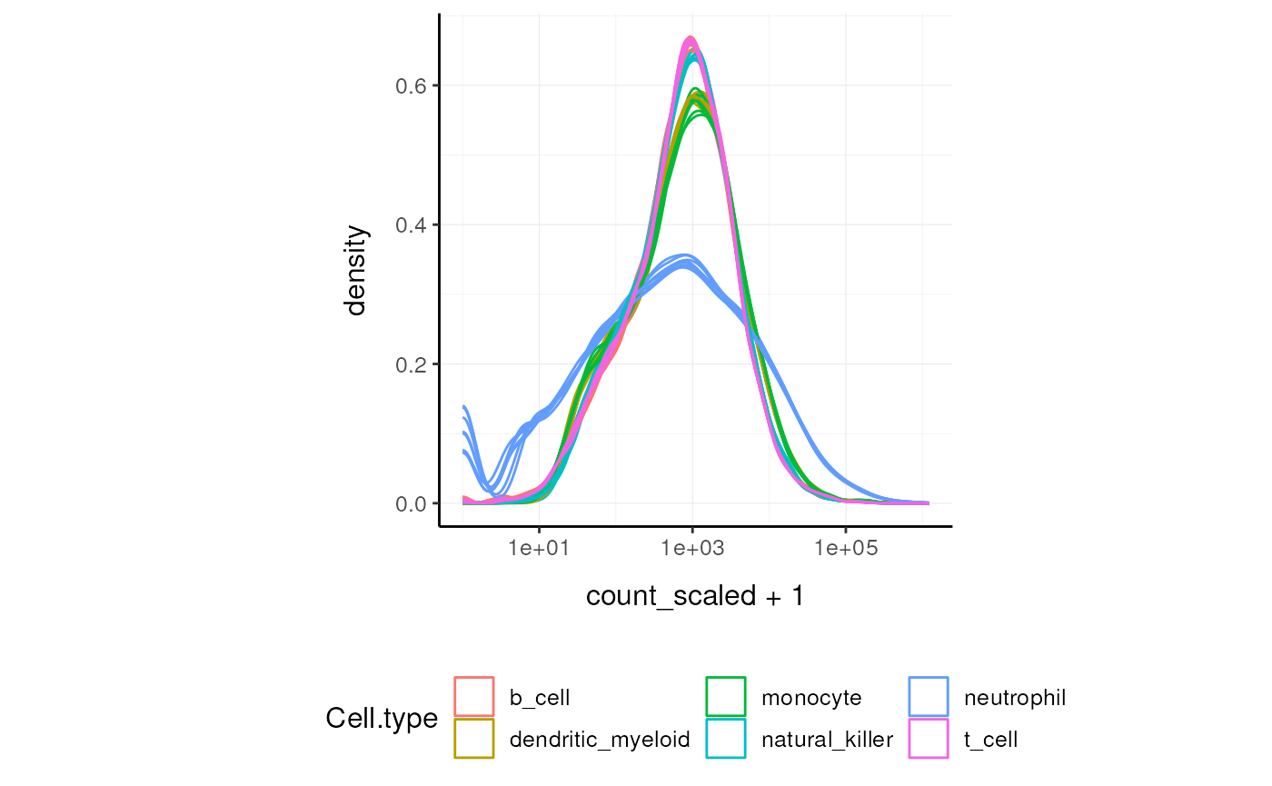
We may want to compensate for sequencing depth, scaling the transcript abundance (e.g., with TMM algorithm, Robinson and Oshlack doi.org/10.1186/gb-2010-11-3-r25). scale_abundance takes a tibble, column names (as symbols; for sample,transcript and count) and a method as arguments and returns a tibble with additional columns with scaled data as <NAME OF COUNT COLUMN>_scaled.

TidyTranscriptomics

## tidybulk says: the sample with largest library size SRR1740035 was chosen as reference for scaling

Standard procedure (comparative purpose)

library(edgeR)

dgList <- DGEList(count_m=x,group=group)
keep <- filterByExpr(dgList)
dgList <- dgList[keep,,keep.lib.sizes=FALSE]
[...]
dgList <- calcNormFactors(dgList, method="TMM")
norm_counts.table <- cpm(dgList)

We can easily plot the scaled density to check the scaling outcome. On the x axis we have the log scaled counts, on the y axes we have the density, data is grouped by sample and coloured by cell type.

Filter `variable transcripts`

We may want to identify and filter variable transcripts.

TidyTranscriptomics

## Getting the 394 most variable genes

Standard procedure (comparative purpose)

library(edgeR)

x = norm_counts.table

s <- rowMeans((x-rowMeans(x))^2)
o <- order(s,decreasing=TRUE)
x <- x[o[1L:top],,drop=FALSE]

norm_counts.table = norm_counts.table[rownames(x)]

norm_counts.table$cell_type = tibble_counts[
    match(
        tibble_counts$sample,
        rownames(norm_counts.table)
    ),
    "Cell.type"
]

Reduce `dimensions`

We may want to reduce the dimensions of our data, for example using PCA or MDS algorithms. reduce_dimensions takes a tibble, column names (as symbols; for sample,transcript and count) and a method (e.g., MDS or PCA) as arguments and returns a tibble with additional columns for the reduced dimensions.

MDS (Robinson et al., 10.1093/bioinformatics/btp616)

TidyTranscriptomics

## Getting the 394 most variable genes

## tidybulk says: to access the raw results do `attr(..., "internals")$MDS`

Standard procedure (comparative purpose)

library(limma)

count_m_log = log(count_m + 1)
cmds = limma::plotMDS(ndim = .dims, plot = FALSE)

cmds = cmds %$% 
    cmdscale.out |>
    setNames(sprintf("Dim%s", 1:6))

cmds$cell_type = tibble_counts[
    match(tibble_counts$sample, rownames(cmds)),
    "Cell.type"
]

On the x and y axes axis we have the reduced dimensions 1 to 3, data is coloured by cell type.

PCA

Standard procedure (comparative purpose)

count_m_log = log(count_m + 1)
pc = count_m_log |> prcomp(scale = TRUE)
variance = pc$sdev^2
variance = (variance / sum(variance))[1:6]
pc$cell_type = counts[
    match(counts$sample, rownames(pc)),
    "Cell.type"
]

On the x and y axes axis we have the reduced dimensions 1 to 3, data is coloured by cell type.

tSNE

Standard procedure (comparative purpose)

count_m_log = log(count_m + 1)

tsne = Rtsne::Rtsne(
    t(count_m_log),
    perplexity=10,
        pca_scale =TRUE
)$Y
tsne$cell_type = tibble_counts[
    match(tibble_counts$sample, rownames(tsne)),
    "Cell.type"
]

Plot

## # A tibble: 251 × 4
##      tSNE1  tSNE2 .sample                      Call 
##      <dbl>  <dbl> <chr>                        <fct>
##  1   0.769  -8.96 TCGA-A1-A0SD-01A-11R-A115-07 LumA 
##  2   7.38    5.86 TCGA-A1-A0SF-01A-11R-A144-07 LumA 
##  3   0.313 -15.3  TCGA-A1-A0SG-01A-11R-A144-07 LumA 
##  4  -5.40   -2.71 TCGA-A1-A0SH-01A-11R-A084-07 LumA 
##  5  -1.30   -4.84 TCGA-A1-A0SI-01A-11R-A144-07 LumB 
##  6   4.18   12.4  TCGA-A1-A0SJ-01A-11R-A084-07 LumA 
##  7  -5.31   27.6  TCGA-A1-A0SK-01A-12R-A084-07 Basal
##  8 -10.7     2.40 TCGA-A1-A0SM-01A-11R-A084-07 LumA 
##  9 -11.4     1.40 TCGA-A1-A0SN-01A-11R-A144-07 LumB 
## 10   2.58  -22.0  TCGA-A1-A0SQ-01A-21R-A144-07 LumA 
## # ℹ 241 more rows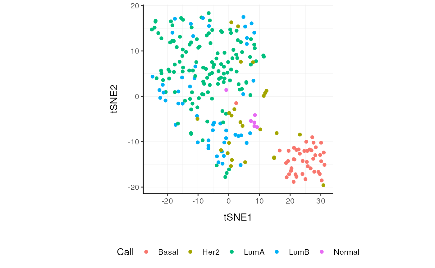

Rotate `dimensions`

We may want to rotate the reduced dimensions (or any two numeric columns really) of our data, of a set angle. rotate_dimensionstakes a tibble, column names (as symbols; for sample,transcript and count) and an angle as arguments and returns a tibble with additional columns for the rotated dimensions. The rotated dimensions will be added to the original data set as <NAME OF DIMENSION> rotated <ANGLE> by default, or as specified in the input arguments.

TidyTranscriptomics

se_mini.norm.MDS.rotated =
  se_mini.norm.MDS |>
    rotate_dimensions(`Dim1`, `Dim2`, rotation_degrees = 45, action="get")

Standard procedure (comparative purpose)

rotation = function(m, d) {
    r = d * pi / 180
    ((bind_rows(
        c(`1` = cos(r), `2` = -sin(r)),
        c(`1` = sin(r), `2` = cos(r))
    ) |> as_matrix()) %*% m)
}
mds_r = pca |> rotation(rotation_degrees)
mds_r$cell_type = counts[
    match(counts$sample, rownames(mds_r)),
    "Cell.type"
]

Original On the x and y axes axis we have the first two reduced dimensions, data is coloured by cell type.

se_mini.norm.MDS.rotated |>
    ggplot(aes(x=`Dim1`, y=`Dim2`, color=`Cell.type` )) +
  geom_point() +
  my_theme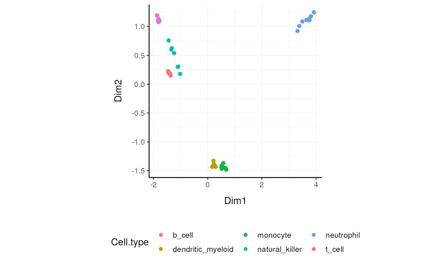

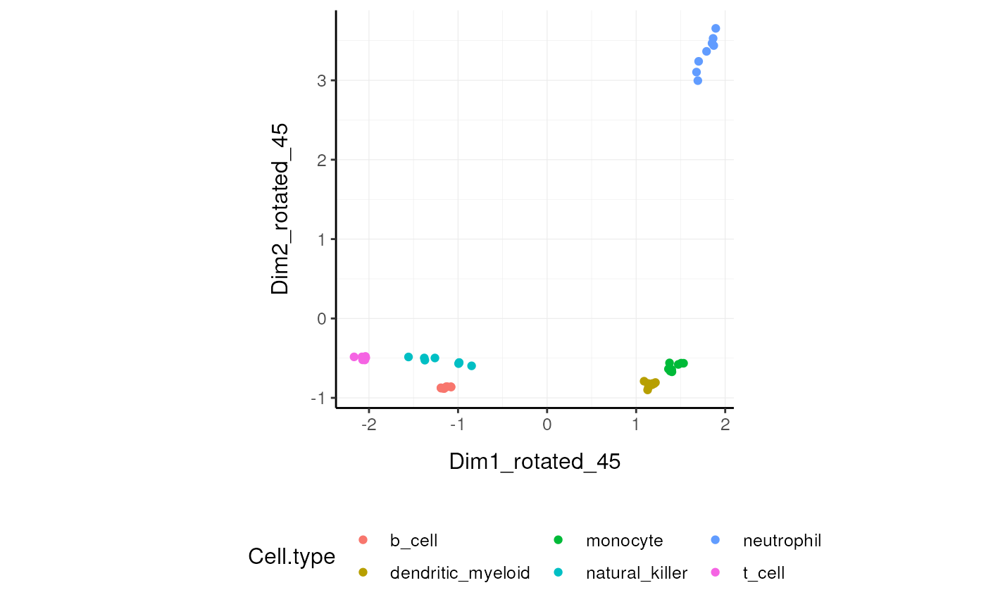
Rotated On the x and y axes axis we have the first two reduced dimensions rotated of 45 degrees, data is coloured by cell type.

Test `differential abundance`

We may want to test for differential transcription between sample-wise factors of interest (e.g., with edgeR).test_differential_abundance takes a tibble, column names (as symbols; for sample, transcript andcount) and a formula representing the desired linear model as arguments and returns a tibble with additional columns for the statistics from the hypothesis test (e.g., log fold change, p-value and false discovery rate).

Standard procedure (comparative purpose)

The functon test_differential_abundance operated with contrasts too. The constrasts hve the name of the design matrix (generally )

Adjust `counts`

We may want to adjust counts for (known) unwanted variation. adjust_abundance takes as arguments a tibble, column names (as symbols; for sample,transcript and count) and a formula representing the desired linear model where the first covariate is the factor of interest and the second covariate is the unwanted variation, and returns a tibble with additional columns for the adjusted counts as<COUNT COLUMN>_adjusted. At the moment just an unwanted covariates is allowed at a time.

TidyTranscriptomics

se_mini.norm.adj =
    se_mini.norm    |> adjust_abundance(    .factor_unwanted = time, .factor_of_interest = condition, method="combat")

Standard procedure (comparative purpose)

library(sva)

count_m_log = log(count_m + 1)

design =
        model.matrix(
            object = ~ factor_of_interest + batch,
            data = annotation
        )

count_m_log.sva =
    ComBat(
            batch = design[,2],
            mod = design,
            ...
        )

count_m_log.sva = ceiling(exp(count_m_log.sva) -1)
count_m_log.sva$cell_type = counts[
    match(counts$sample, rownames(count_m_log.sva)),
    "Cell.type"
]

Deconvolve `Cell type composition`

We may want to infer the cell type composition of our samples (with the algorithm Cibersort; Newman et al., 10.1038/nmeth.3337).deconvolve_cellularity takes as arguments a tibble, column names (as symbols; for sample, transcript andcount) and returns a tibble with additional columns for the adjusted cell type proportions.

Standard procedure (comparative purpose)

source(‘CIBERSORT.R’)
count_m |> write.table("mixture_file.txt")
results <- CIBERSORT(
    "sig_matrix_file.txt",
    "mixture_file.txt",
    perm=100, QN=TRUE
)
results$cell_type = tibble_counts[
    match(tibble_counts$sample, rownames(results)),
    "Cell.type"
]

With the new annotated data frame, we can plot the distributions of cell types across samples, and compare them with the nominal cell type labels to check for the purity of isolation. On the x axis we have the cell types inferred by Cibersort, on the y axis we have the inferred proportions. The data is facetted and coloured by nominal cell types (annotation given by the researcher after FACS sorting).

se_mini.cibersort |>
    pivot_longer(
        names_to= "Cell_type_inferred", 
        values_to = "proportion", 
        names_prefix ="cibersort__", 
        cols=contains("cibersort__")
    ) |>
  ggplot(aes(x=Cell_type_inferred, y=proportion, fill=`Cell.type`)) +
  geom_boxplot() +
  facet_wrap(~`Cell.type`) +
  my_theme +
  theme(axis.text.x = element_text(angle = 90, hjust = 1, vjust = 0.5), aspect.ratio=1/5)

Test differential cell-type abundance

We can also perform a statistical test on the differential cell-type abundance across conditions

We can also perform regression analysis with censored data (coxph).

Cluster `samples`

We may want to cluster our data (e.g., using k-means sample-wise).cluster_elements takes as arguments a tibble, column names (as symbols; for sample, transcript andcount) and returns a tibble with additional columns for the cluster annotation. At the moment only k-means clustering is supported, the plan is to introduce more clustering methods.

k-means

TidyTranscriptomics

se_mini.norm.cluster = se_mini.norm.MDS |>
  cluster_elements(method="kmeans", centers = 2, action="get" )

Standard procedure (comparative purpose)

count_m_log = log(count_m + 1)

k = kmeans(count_m_log, iter.max = 1000, ...)
cluster = k$cluster

cluster$cell_type = tibble_counts[
    match(tibble_counts$sample, rownames(cluster)),
    c("Cell.type", "Dim1", "Dim2")
]

We can add cluster annotation to the MDS dimension reduced data set and plot.

 se_mini.norm.cluster |>
    ggplot(aes(x=`Dim1`, y=`Dim2`, color=`cluster_kmeans`)) +
  geom_point() +
  my_theme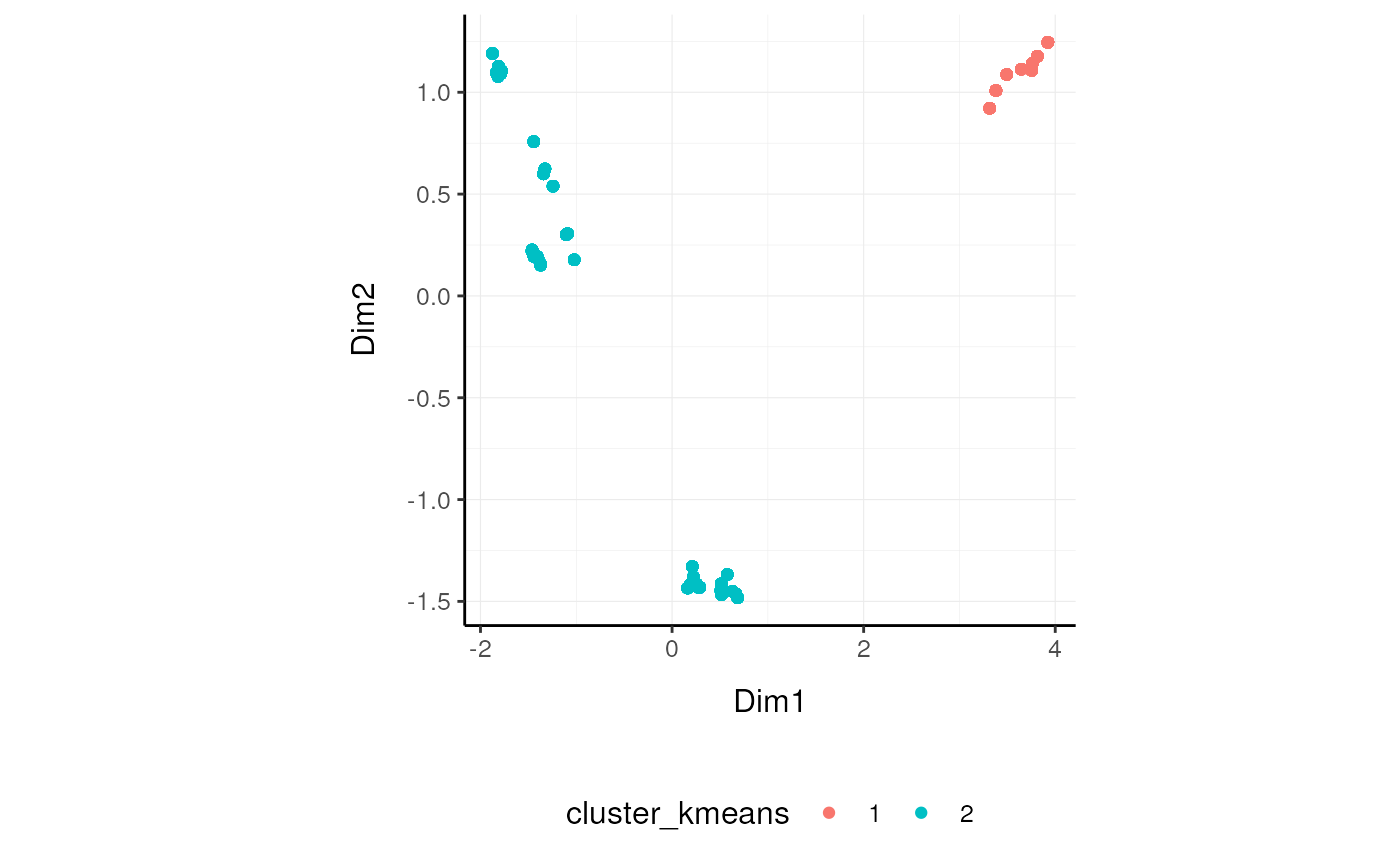

SNN

Matrix package (v1.3-3) causes an error with Seurat::FindNeighbors used in this method. We are trying to solve this issue. At the moment this option in unaviable.

Standard procedure (comparative purpose)

library(Seurat)

snn = CreateSeuratObject(count_m)
snn = ScaleData(
    snn, display.progress = TRUE,
    num.cores=4, do.par = TRUE
)
snn = FindVariableFeatures(snn, selection.method = "vst")
snn = FindVariableFeatures(snn, selection.method = "vst")
snn = RunPCA(snn, npcs = 30)
snn = FindNeighbors(snn)
snn = FindClusters(snn, method = "igraph", ...)
snn = snn[["seurat_clusters"]]

snn$cell_type = tibble_counts[
    match(tibble_counts$sample, rownames(snn)),
    c("Cell.type", "Dim1", "Dim2")
]

Drop `redundant` transcripts

We may want to remove redundant elements from the original data set (e.g., samples or transcripts), for example if we want to define cell-type specific signatures with low sample redundancy.remove_redundancy takes as arguments a tibble, column names (as symbols; for sample, transcript andcount) and returns a tibble with redundant elements removed (e.g., samples). Two redundancy estimation approaches are supported:

removal of highly correlated clusters of elements (keeping a representative) with method=“correlation”
removal of most proximal element pairs in a reduced dimensional space.

Approach 1

TidyTranscriptomics

se_mini.norm.non_redundant =
    se_mini.norm.MDS |>
  remove_redundancy(    method = "correlation" )

## Getting the 394 most variable genes

Standard procedure (comparative purpose)

library(widyr)

.data.correlated =
    pairwise_cor(
        counts,
        sample,
        transcript,
        rc,
        sort = TRUE,
        diag = FALSE,
        upper = FALSE
    ) |>
    filter(correlation > correlation_threshold) |>
    distinct(item1) |>
    rename(!!.element := item1)

# Return non redudant data frame
counts |> anti_join(.data.correlated) |>
    spread(sample, rc, - transcript) |>
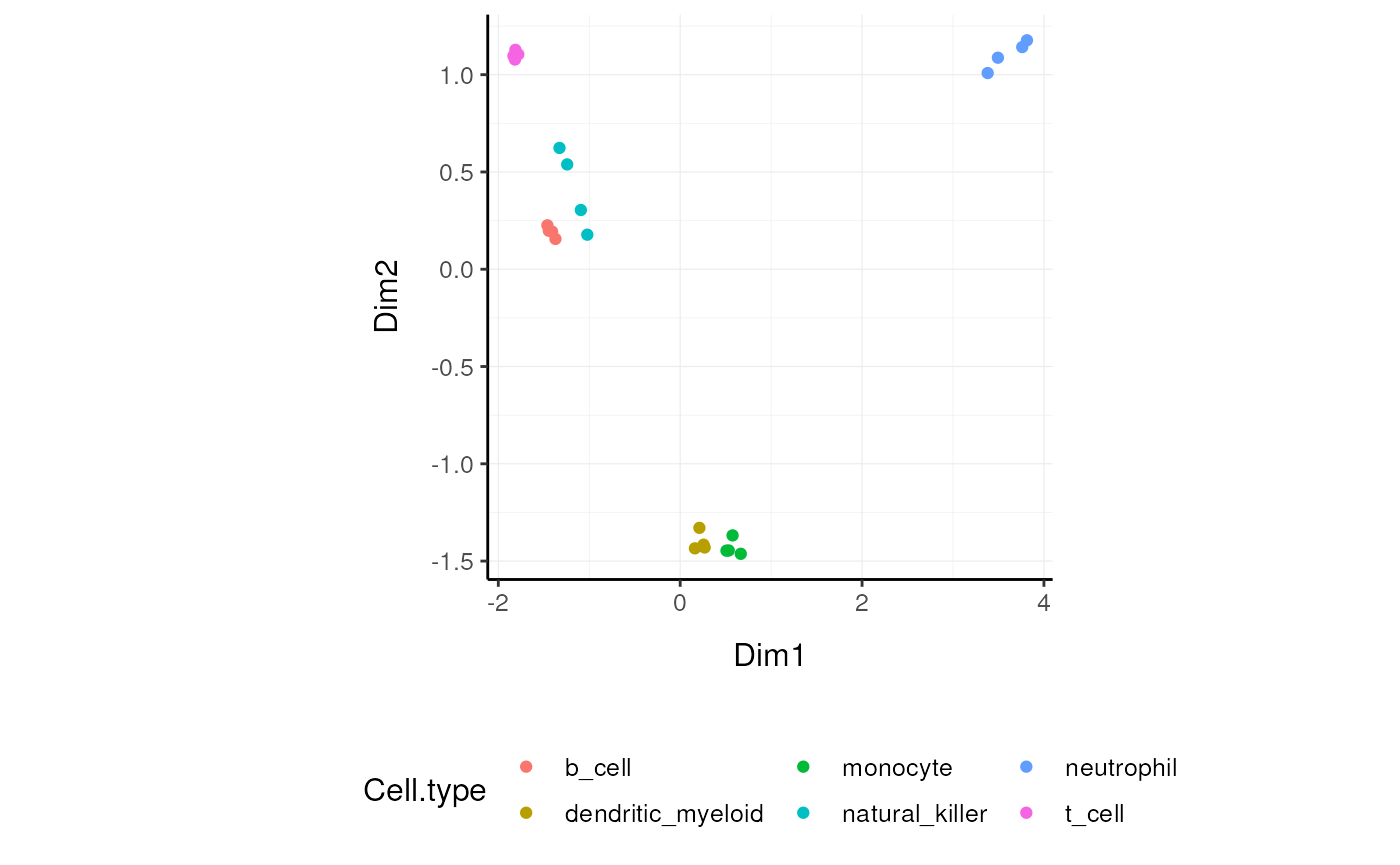
    left_join(annotation)

We can visualise how the reduced redundancy with the reduced dimentions look like

Approach 2

se_mini.norm.non_redundant =
    se_mini.norm.MDS |>
  remove_redundancy(
    method = "reduced_dimensions",
    Dim_a_column = `Dim1`,
    Dim_b_column = `Dim2`
  )

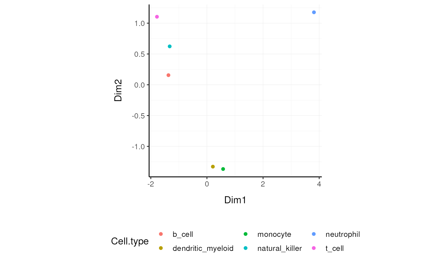
We can visualise MDS reduced dimensions of the samples with the closest pair removed.

Other useful wrappers

The above wrapper streamline the most common processing of bulk RNA sequencing data. Other useful wrappers are listed above.

From BAM/SAM to tibble of gene counts

We can calculate gene counts (using FeatureCounts; Liao Y et al., 10.1093/nar/gkz114) from a list of BAM/SAM files and format them into a tidy structure (similar to counts).

counts = tidybulk_SAM_BAM(
    file_names,
    genome = "hg38",
    isPairedEnd = TRUE,
    requireBothEndsMapped = TRUE,
    checkFragLength = FALSE,
    useMetaFeatures = TRUE
)

From ensembl IDs to gene symbol IDs

We can add gene symbols from ensembl identifiers. This is useful since different resources use ensembl IDs while others use gene symbol IDs. This currently works for human and mouse.

## # A tibble: 119 × 8
##    ens   iso   `read count` sample cases_0_project_dise…¹ cases_0_samples_0_sa…²
##    <chr> <chr>        <dbl> <chr>  <chr>                  <chr>                 
##  1 ENSG… 13             144 TARGE… Acute Myeloid Leukemia Primary Blood Derived…
##  2 ENSG… 13              72 TARGE… Acute Myeloid Leukemia Primary Blood Derived…
##  3 ENSG… 13               0 TARGE… Acute Myeloid Leukemia Primary Blood Derived…
##  4 ENSG… 13            1099 TARGE… Acute Myeloid Leukemia Primary Blood Derived…
##  5 ENSG… 13              11 TARGE… Acute Myeloid Leukemia Primary Blood Derived…
##  6 ENSG… 13               2 TARGE… Acute Myeloid Leukemia Primary Blood Derived…
##  7 ENSG… 13               3 TARGE… Acute Myeloid Leukemia Primary Blood Derived…
##  8 ENSG… 13            2678 TARGE… Acute Myeloid Leukemia Primary Blood Derived…
##  9 ENSG… 13             751 TARGE… Acute Myeloid Leukemia Primary Blood Derived…
## 10 ENSG… 13               1 TARGE… Acute Myeloid Leukemia Primary Blood Derived…
## # ℹ 109 more rows
## # ℹ abbreviated names: ¹cases_0_project_disease_type,
## #   ²cases_0_samples_0_sample_type
## # ℹ 2 more variables: transcript <chr>, ref_genome <chr>

From gene symbol to gene description (gene name in full)

We can add gene full name (and in future description) from symbol identifiers. This currently works for human and mouse.

##

##

## Warning in is_sample_feature_deprecated_used(.data, .cols):
## tidySummarizedExperiment says: from version 1.3.1, the special columns
## including sample/feature id (colnames(se), rownames(se)) has changed to
## ".sample" and ".feature". This dataset is returned with the old-style
## vocabulary (feature and sample), however we suggest to update your workflow to
## reflect the new vocabulary (.feature, .sample)

## # A SummarizedExperiment-tibble abstraction: 2,635 × 11
## # Features=527 | Samples=5 | Assays=count
##    feature sample count Cell.type time  condition  days  dead description entrez
##    <chr>   <chr>  <dbl> <chr>     <chr> <lgl>     <dbl> <dbl> <chr>       <chr> 
##  1 ABCB4   SRR17…  1035 b_cell    0 d   TRUE          1     1 ATP bindin… 5244  
##  2 ABCB9   SRR17…    45 b_cell    0 d   TRUE          1     1 ATP bindin… 23457 
##  3 ACAP1   SRR17…  7151 b_cell    0 d   TRUE          1     1 ArfGAP wit… 9744  
##  4 ACHE    SRR17…     2 b_cell    0 d   TRUE          1     1 acetylchol… 43    
##  5 ACP5    SRR17…  2278 b_cell    0 d   TRUE          1     1 acid phosp… 54    
##  6 ADAM28  SRR17… 11156 b_cell    0 d   TRUE          1     1 ADAM metal… 10863 
##  7 ADAMDE… SRR17…    72 b_cell    0 d   TRUE          1     1 ADAM like … 27299 
##  8 ADAMTS3 SRR17…     0 b_cell    0 d   TRUE          1     1 ADAM metal… 9508  
##  9 ADRB2   SRR17…   298 b_cell    0 d   TRUE          1     1 adrenocept… 154   
## 10 AIF1    SRR17…     8 b_cell    0 d   TRUE          1     1 allograft … 199   
## # ℹ 40 more rows
## # ℹ 1 more variable: gene_name <chr>

Appendix

## R Under development (unstable) (2025-03-08 r87910)
## Platform: x86_64-pc-linux-gnu
## Running under: Ubuntu 24.04.1 LTS
## 
## Matrix products: default
## BLAS:   /usr/lib/x86_64-linux-gnu/openblas-pthread/libblas.so.3 
## LAPACK: /usr/lib/x86_64-linux-gnu/openblas-pthread/libopenblasp-r0.3.26.so;  LAPACK version 3.12.0
## 
## locale:
##  [1] LC_CTYPE=en_US.UTF-8       LC_NUMERIC=C              
##  [3] LC_TIME=en_US.UTF-8        LC_COLLATE=en_US.UTF-8    
##  [5] LC_MONETARY=en_US.UTF-8    LC_MESSAGES=en_US.UTF-8   
##  [7] LC_PAPER=en_US.UTF-8       LC_NAME=C                 
##  [9] LC_ADDRESS=C               LC_TELEPHONE=C            
## [11] LC_MEASUREMENT=en_US.UTF-8 LC_IDENTIFICATION=C       
## 
## time zone: UTC
## tzcode source: system (glibc)
## 
## attached base packages:
## [1] stats4    stats     graphics  grDevices utils     datasets  methods  
## [8] base     
## 
## other attached packages:
##  [1] tidySummarizedExperiment_1.17.0 SummarizedExperiment_1.37.0    
##  [3] Biobase_2.67.0                  GenomicRanges_1.59.1           
##  [5] GenomeInfoDb_1.43.4             IRanges_2.41.3                 
##  [7] S4Vectors_0.45.4                BiocGenerics_0.53.6            
##  [9] generics_0.1.3                  MatrixGenerics_1.19.1          
## [11] matrixStats_1.5.0               tidybulk_1.19.3                
## [13] ttservice_0.4.1                 ggrepel_0.9.6                  
## [15] ggplot2_3.5.1                   magrittr_2.0.3                 
## [17] tibble_3.2.1                    tidyr_1.3.1                    
## [19] dplyr_1.1.4                     knitr_1.50                     
## [21] BiocStyle_2.35.0               
## 
## loaded via a namespace (and not attached):
##   [1] jsonlite_2.0.0          farver_2.1.2            rmarkdown_2.29         
##   [4] fs_1.6.5                ragg_1.3.3              vctrs_0.6.5            
##   [7] memoise_2.0.1           htmltools_0.5.8.1       S4Arrays_1.7.3         
##  [10] broom_1.0.8             janeaustenr_1.0.0       SparseArray_1.7.7      
##  [13] sass_0.4.9              bslib_0.9.0             htmlwidgets_1.6.4      
##  [16] tokenizers_0.3.0        desc_1.4.3              plyr_1.8.9             
##  [19] plotly_4.10.4           cachem_1.1.0            lifecycle_1.0.4        
##  [22] pkgconfig_2.0.3         Matrix_1.7-3            R6_2.6.1               
##  [25] fastmap_1.2.0           GenomeInfoDbData_1.2.14 digest_0.6.37          
##  [28] tidytext_0.4.2          colorspace_2.1-1        AnnotationDbi_1.69.0   
##  [31] textshaping_1.0.0       SnowballC_0.7.1         RSQLite_2.3.9          
##  [34] org.Hs.eg.db_3.21.0     labeling_0.4.3          org.Mm.eg.db_3.21.0    
##  [37] fansi_1.0.6             httr_1.4.7              abind_1.4-8            
##  [40] mgcv_1.9-3              compiler_4.5.0          proxy_0.4-27           
##  [43] bit64_4.6.0-1           withr_3.0.2             backports_1.5.0        
##  [46] BiocParallel_1.41.5     DBI_1.2.3               DelayedArray_0.33.6    
##  [49] tools_4.5.0             glue_1.8.0              nlme_3.1-168           
##  [52] grid_4.5.0              Rtsne_0.17              reshape2_1.4.4         
##  [55] sva_3.55.0              gtable_0.3.6            tzdb_0.5.0             
##  [58] class_7.3-23            preprocessCore_1.69.0   data.table_1.17.0      
##  [61] hms_1.1.3               utf8_1.2.4              XVector_0.47.2         
##  [64] pillar_1.10.2           stringr_1.5.1           limma_3.63.11          
##  [67] genefilter_1.89.0       splines_4.5.0           lattice_0.22-7         
##  [70] survival_3.8-3          bit_4.6.0               annotate_1.85.0        
##  [73] tidyselect_1.2.1        locfit_1.5-9.12         Biostrings_2.75.4      
##  [76] bookdown_0.42           edgeR_4.5.10            xfun_0.52              
##  [79] statmod_1.5.0           stringi_1.8.7           UCSC.utils_1.3.1       
##  [82] lazyeval_0.2.2          yaml_2.3.10             evaluate_1.0.3         
##  [85] codetools_0.2-20        widyr_0.1.5             BiocManager_1.30.25    
##  [88] cli_3.6.4               xtable_1.8-4            systemfonts_1.2.2      
##  [91] munsell_0.5.1           jquerylib_0.1.4         Rcpp_1.0.14            
##  [94] png_0.1-8               XML_3.99-0.18           parallel_4.5.0         
##  [97] ellipsis_0.3.2          pkgdown_2.1.1           readr_2.1.5            
## [100] blob_1.2.4              viridisLite_0.4.2       scales_1.3.0           
## [103] e1071_1.7-16            purrr_1.0.4             crayon_1.5.3           
## [106] rlang_1.1.5             KEGGREST_1.47.0

Overview of the tidybulk package (original) (raw)

Data

Get the bibliography of your workflow

Aggregate duplicated transcripts

Scale counts

Filter variable transcripts

Reduce dimensions

Rotate dimensions

Test differential abundance

Adjust counts

Deconvolve Cell type composition

Test differential cell-type abundance

Cluster samples

Drop redundant transcripts

Other useful wrappers

From BAM/SAM to tibble of gene counts

From ensembl IDs to gene symbol IDs

From gene symbol to gene description (gene name in full)

Appendix

Aggregate duplicated `transcripts`

Scale `counts`

Filter `variable transcripts`

Reduce `dimensions`

Rotate `dimensions`

Test `differential abundance`

Adjust `counts`

Deconvolve `Cell type composition`

Cluster `samples`

Drop `redundant` transcripts