Overview of the tidyseurat package (original) (raw)
![]()
Brings Seurat to the tidyverse!
website: stemangiola.github.io/tidyseurat/
Please also have a look at
- tidyseuratfor tidy single-cell RNA sequencing analysis
- tidySummarizedExperimentfor tidy bulk RNA sequencing analysis
- tidybulk for tidy bulk RNA-seq analysis
- nanny for tidy high-level data analysis and manipulation
- tidygate for adding custom gate information to your tibble
- tidyHeatmapfor heatmaps produced with tidy principles
![]()
visual cue
Introduction
tidyseurat provides a bridge between the Seurat single-cell package(Butler et al. 2018; Stuart et al. 2019)and the tidyverse (Wickham et al. 2019). It creates an invisible layer that enables viewing the Seurat object as a tidyverse tibble, and provides Seurat-compatible dplyr,tidyr, ggplot and plotly functions.
Functions/utilities available
| Seurat-compatible Functions | Description |
|---|---|
| all |
| tidyverse Packages | Description |
|---|---|
| dplyr | All dplyr APIs like for any tibble |
| tidyr | All tidyr APIs like for any tibble |
| ggplot2 | ggplot like for any tibble |
| plotly | plot_ly like for any tibble |
| Utilities | Description |
|---|---|
| tidy | Add tidyseurat invisible layer over a Seurat object |
| as_tibble | Convert cell-wise information to a tbl_df |
| join_features | Add feature-wise information, returns a tbl_df |
| aggregate_cells | Aggregate cell gene-transcription abundance as pseudobulk tissue |
Installation
From CRAN
From Github (development)
Create tidyseurat, the best of both worlds
This is a seurat object but it is evaluated as tibble. So it is fully compatible both with Seurat and tidyverse APIs.
It looks like a tibble
## # A Seurat-tibble abstraction: 80 × 15
## # Features=230 | Cells=80 | Active assay=RNA | Assays=RNA
##    .cell orig.ident nCount_RNA nFeature_RNA RNA_snn_res.0.8 letter.idents groups
##    <chr> <fct>           <dbl>        <int> <fct>           <fct>         <chr>
##  1 ATGC… SeuratPro…         70           47 0               A             g2
##  2 CATG… SeuratPro…         85           52 0               A             g1
##  3 GAAC… SeuratPro…         87           50 1               B             g2
##  4 TGAC… SeuratPro…        127           56 0               A             g2
##  5 AGTC… SeuratPro…        173           53 0               A             g2
##  6 TCTG… SeuratPro…         70           48 0               A             g1
##  7 TGGT… SeuratPro…         64           36 0               A             g1
##  8 GCAG… SeuratPro…         72           45 0               A             g1
##  9 GATA… SeuratPro…         52           36 0               A             g1
## 10 AATG… SeuratPro…        100           41 0               A             g1
## # ℹ 70 more rows
## # ℹ 8 more variables: RNA_snn_res.1 <fct>, PC_1 <dbl>, PC_2 <dbl>, PC_3 <dbl>,
## #   PC_4 <dbl>, PC_5 <dbl>, tSNE_1 <dbl>, tSNE_2 <dbl>
But it is a Seurat object after all
## $RNA
## Assay data with 230 features for 80 cells
## Top 10 variable features:
##  PPBP, IGLL5, VDAC3, CD1C, AKR1C3, PF4, MYL9, GNLY, TREML1, CA2
Preliminary plots
Set colours and theme for plots.
# Use colourblind-friendly colours
friendly_cols <- c("#88CCEE", "#CC6677", "#DDCC77", "#117733", "#332288", "#AA4499", "#44AA99", "#999933", "#882255", "#661100", "#6699CC")

# Set theme
my_theme <-
  list(
    scale_fill_manual(values = friendly_cols),
    scale_color_manual(values = friendly_cols),
    theme_bw() +
      theme(
        panel.border = element_blank(),
        axis.line = element_line(),
        panel.grid.major = element_line(size = 0.2),
        panel.grid.minor = element_line(size = 0.1),
        text = element_text(size = 12),
        legend.position = "bottom",
        aspect.ratio = 1,
        strip.background = element_blank(),
        axis.title.x = element_text(margin = margin(t = 10, r = 10, b = 10, l = 10)),
        axis.title.y = element_text(margin = margin(t = 10, r = 10, b = 10, l = 10))
      )
  )
We can treat pbmc_small effectively as a normal tibble for plotting.
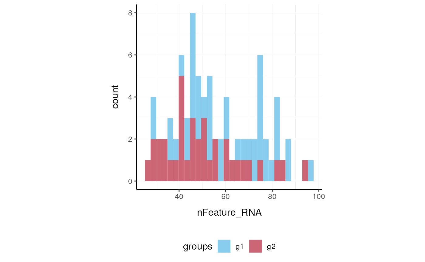
Here we plot number of features per cell.
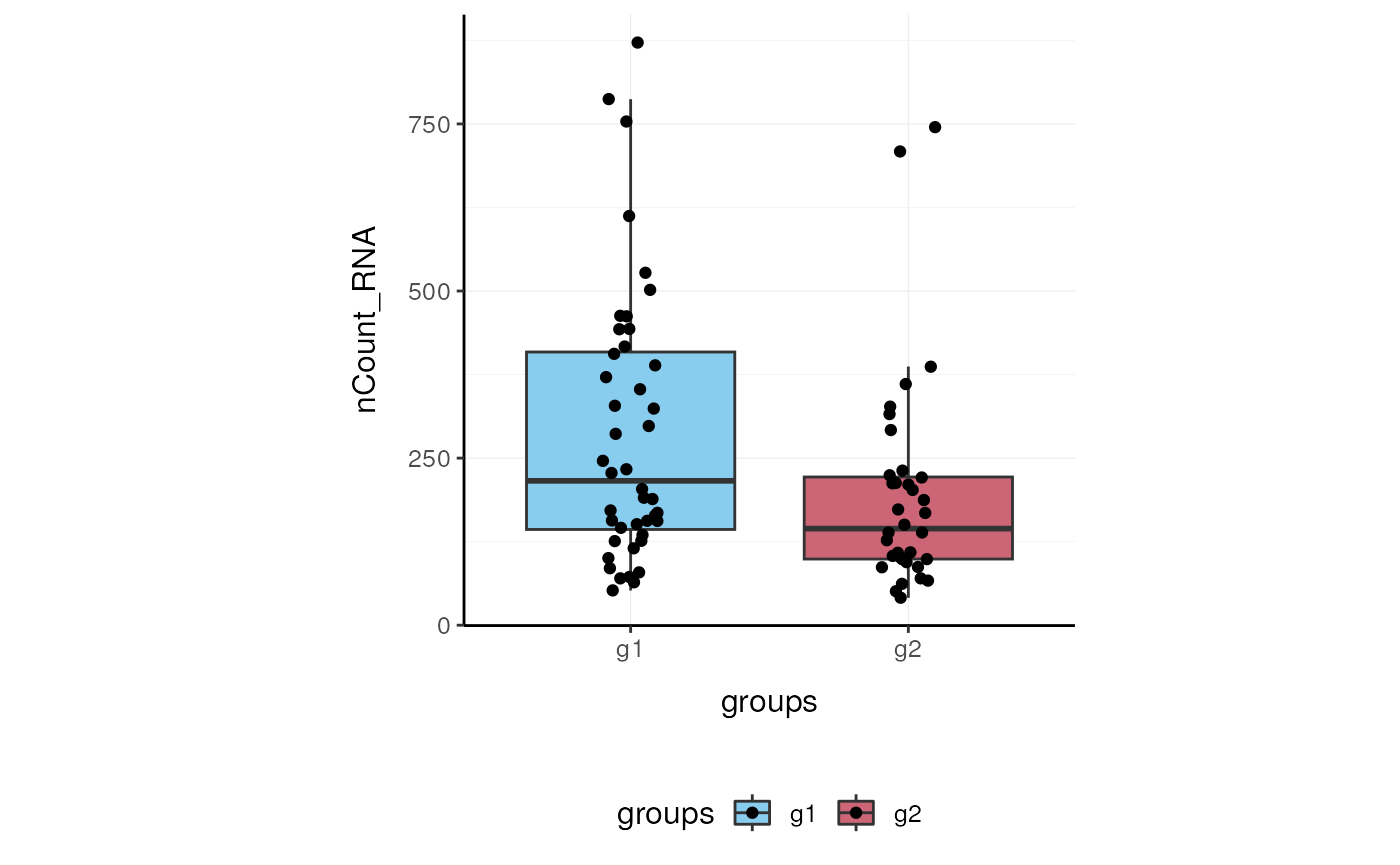
Here we plot total features per cell.
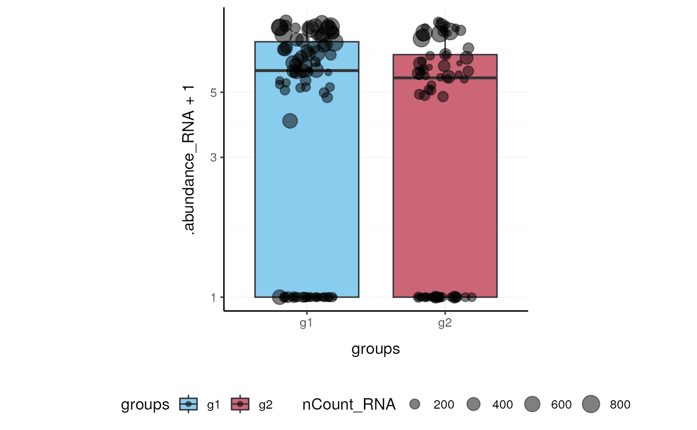
Here we plot abundance of two features for each group.
Preprocess the dataset
Also you can treat the object as Seurat object and proceed with data processing.
## # A Seurat-tibble abstraction: 80 × 17
## # Features=220 | Cells=80 | Active assay=SCT | Assays=RNA, SCT
##    .cell orig.ident nCount_RNA nFeature_RNA RNA_snn_res.0.8 letter.idents groups
##    <chr> <fct>           <dbl>        <int> <fct>           <fct>         <chr>
##  1 ATGC… SeuratPro…         70           47 0               A             g2
##  2 CATG… SeuratPro…         85           52 0               A             g1
##  3 GAAC… SeuratPro…         87           50 1               B             g2
##  4 TGAC… SeuratPro…        127           56 0               A             g2
##  5 AGTC… SeuratPro…        173           53 0               A             g2
##  6 TCTG… SeuratPro…         70           48 0               A             g1
##  7 TGGT… SeuratPro…         64           36 0               A             g1
##  8 GCAG… SeuratPro…         72           45 0               A             g1
##  9 GATA… SeuratPro…         52           36 0               A             g1
## 10 AATG… SeuratPro…        100           41 0               A             g1
## # ℹ 70 more rows
## # ℹ 10 more variables: RNA_snn_res.1 <fct>, nCount_SCT <dbl>,
## #   nFeature_SCT <int>, PC_1 <dbl>, PC_2 <dbl>, PC_3 <dbl>, PC_4 <dbl>,
## #   PC_5 <dbl>, tSNE_1 <dbl>, tSNE_2 <dbl>
If a tool is not included in the tidyseurat collection, we can useas_tibble to permanently convert tidyseuratinto tibble.
Identify clusters
We proceed with cluster identification with Seurat.
## # A Seurat-tibble abstraction: 80 × 19
## # Features=220 | Cells=80 | Active assay=SCT | Assays=RNA, SCT
##    .cell orig.ident nCount_RNA nFeature_RNA RNA_snn_res.0.8 letter.idents groups
##    <chr> <fct>           <dbl>        <int> <fct>           <fct>         <chr>
##  1 ATGC… SeuratPro…         70           47 0               A             g2
##  2 CATG… SeuratPro…         85           52 0               A             g1
##  3 GAAC… SeuratPro…         87           50 1               B             g2
##  4 TGAC… SeuratPro…        127           56 0               A             g2
##  5 AGTC… SeuratPro…        173           53 0               A             g2
##  6 TCTG… SeuratPro…         70           48 0               A             g1
##  7 TGGT… SeuratPro…         64           36 0               A             g1
##  8 GCAG… SeuratPro…         72           45 0               A             g1
##  9 GATA… SeuratPro…         52           36 0               A             g1
## 10 AATG… SeuratPro…        100           41 0               A             g1
## # ℹ 70 more rows
## # ℹ 12 more variables: RNA_snn_res.1 <fct>, nCount_SCT <dbl>,
## #   nFeature_SCT <int>, SCT_snn_res.0.8 <fct>, seurat_clusters <fct>,
## #   PC_1 <dbl>, PC_2 <dbl>, PC_3 <dbl>, PC_4 <dbl>, PC_5 <dbl>, tSNE_1 <dbl>,
## #   tSNE_2 <dbl>
Now we can interrogate the object as if it was a regular tibble data frame.
pbmc_small_cluster %>%
  count(groups, seurat_clusters)
## # A tibble: 6 × 3
## groups seurat_clusters n
## <chr> <fct> <int>
## 1 g1 0 23
## 2 g1 1 17
## 3 g1 2 4
## 4 g2 0 17
## 5 g2 1 13
## 6 g2 2 6We can identify cluster markers using Seurat.
# Identify top 10 markers per cluster
markers <-
  pbmc_small_cluster %>%
  FindAllMarkers(only.pos = TRUE, min.pct = 0.25, thresh.use = 0.25) %>%
  group_by(cluster) %>%
  top_n(10, avg_log2FC)

# Plot heatmap
pbmc_small_cluster %>%
  DoHeatmap(
    features = markers$gene,
    group.colors = friendly_cols
  )
Reduce dimensions
We can calculate the first 3 UMAP dimensions using the Seurat framework.
pbmc_small_UMAP <-
  pbmc_small_cluster %>%
  RunUMAP(reduction = "pca", dims = 1:15, n.components = 3L)
And we can plot them using 3D plot using plotly.
pbmc_small_UMAP %>%
  plot_ly(
    x = ~`UMAP_1`,
    y = ~`UMAP_2`,
    z = ~`UMAP_3`,
    color = ~seurat_clusters,
    colors = friendly_cols[1:4]
  )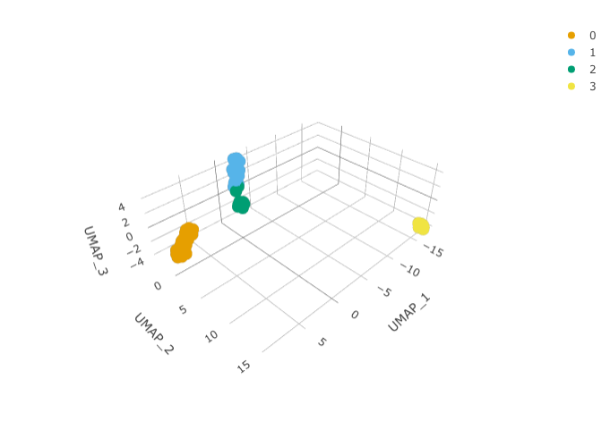
screenshot plotly
Cell type prediction
We can infer cell type identities using SingleR (Aran et al. 2019) and manipulate the output using tidyverse.
# Get cell type reference data
blueprint <- celldex::BlueprintEncodeData()

# Infer cell identities
cell_type_df <-
  GetAssayData(pbmc_small_UMAP, slot = 'counts', assay = "SCT") %>%
  log1p() %>%
  Matrix::Matrix(sparse = TRUE) %>%
  SingleR::SingleR(
    ref = blueprint,
    labels = blueprint$label.main,
    method = "single"
  ) %>%
  as.data.frame() %>%
  as_tibble(rownames = "cell") %>%
  select(cell, first.labels)
# Join UMAP and cell type info
pbmc_small_cell_type <-
pbmc_small_UMAP %>%
left_join(cell_type_df, by = "cell")
# Reorder columns
pbmc_small_cell_type %>%
select(cell, first.labels, everything())We can easily summarise the results. For example, we can see how cell type classification overlaps with cluster classification.
pbmc_small_cell_type %>%
  count(seurat_clusters, first.labels)
We can easily reshape the data for building information-rich faceted plots.
pbmc_small_cell_type %>%

  # Reshape and add classifier column
  pivot_longer(
    cols = c(seurat_clusters, first.labels),
    names_to = "classifier", values_to = "label"
  ) %>%

  # UMAP plots for cell type and cluster
  ggplot(aes(UMAP_1, UMAP_2, color = label)) +
  geom_point() +
  facet_wrap(~classifier) +
  my_theme
We can easily plot gene correlation per cell category, adding multi-layer annotations.
Nested analyses
A powerful tool we can use with tidyseurat is nest. We can easily perform independent analyses on subsets of the dataset. First we classify cell types in lymphoid and myeloid; then, nest based on the new classification
pbmc_small_nested <-
  pbmc_small_cell_type %>%
  filter(first.labels != "Erythrocytes") %>%
  mutate(cell_class = if_else(`first.labels` %in% c("Macrophages", "Monocytes"), "myeloid", "lymphoid")) %>%
  nest(data = -cell_class)

pbmc_small_nested
Now we can independently for the lymphoid and myeloid subsets (i) find variable features, (ii) reduce dimensions, and (iii) cluster using both tidyverse and Seurat seamlessly.
Now we can unnest and plot the new classification.
pbmc_small_nested_reanalysed %>%

  # Convert to tibble otherwise Seurat drops reduced dimensions when unifying data sets.
  mutate(data = map(data, ~ .x %>% as_tibble())) %>%
  unnest(data) %>%

  # Define unique clusters
  unite("cluster", c(cell_class, seurat_clusters), remove = FALSE) %>%

  # Plotting
  ggplot(aes(UMAP_1, UMAP_2, color = cluster)) +
  geom_point() +
  facet_wrap(~cell_class) +
  my_theme
Aggregating cells
Sometimes, it is necessary to aggregate the gene-transcript abundance from a group of cells into a single value. For example, when comparing groups of cells across different samples with fixed-effect models.
In tidyseurat, cell aggregation can be achieved using theaggregate_cells function.
Session Info
## R version 4.4.1 (2024-06-14)
## Platform: x86_64-pc-linux-gnu
## Running under: Ubuntu 22.04.4 LTS
##
## Matrix products: default
## BLAS:   /usr/lib/x86_64-linux-gnu/openblas-pthread/libblas.so.3
## LAPACK: /usr/lib/x86_64-linux-gnu/openblas-pthread/libopenblasp-r0.3.20.so;  LAPACK version 3.10.0
##
## locale:
##  [1] LC_CTYPE=en_US.UTF-8       LC_NUMERIC=C
##  [3] LC_TIME=en_US.UTF-8        LC_COLLATE=en_US.UTF-8
##  [5] LC_MONETARY=en_US.UTF-8    LC_MESSAGES=en_US.UTF-8
##  [7] LC_PAPER=en_US.UTF-8       LC_NAME=C
##  [9] LC_ADDRESS=C               LC_TELEPHONE=C
## [11] LC_MEASUREMENT=en_US.UTF-8 LC_IDENTIFICATION=C
##
## time zone: UTC
## tzcode source: system (glibc)
##
## attached base packages:
## [1] stats     graphics  grDevices utils     datasets  methods   base
##
## other attached packages:
##  [1] tidyseurat_0.8.2   ttservice_0.4.1    Seurat_5.1.0       SeuratObject_5.0.2
##  [5] sp_2.1-4           ggplot2_3.5.1      magrittr_2.0.3     purrr_1.0.2
##  [9] tidyr_1.3.1        dplyr_1.1.4        knitr_1.48
##
## loaded via a namespace (and not attached):
##   [1] RColorBrewer_1.1-3     jsonlite_1.8.8         spatstat.utils_3.0-5
##   [4] farver_2.1.2           rmarkdown_2.27         fs_1.6.4
##   [7] ragg_1.3.2             vctrs_0.6.5            ROCR_1.0-11
##  [10] spatstat.explore_3.3-1 htmltools_0.5.8.1      sass_0.4.9
##  [13] sctransform_0.4.1      parallelly_1.37.1      KernSmooth_2.23-24
##  [16] bslib_0.7.0            htmlwidgets_1.6.4      desc_1.4.3
##  [19] ica_1.0-3              plyr_1.8.9             plotly_4.10.4
##  [22] zoo_1.8-12             cachem_1.1.0           igraph_2.0.3
##  [25] mime_0.12              lifecycle_1.0.4        pkgconfig_2.0.3
##  [28] Matrix_1.7-0           R6_2.5.1               fastmap_1.2.0
##  [31] fitdistrplus_1.2-1     future_1.33.2          shiny_1.8.1.1
##  [34] digest_0.6.36          GGally_2.2.1           colorspace_2.1-0
##  [37] patchwork_1.2.0        tensor_1.5             RSpectra_0.16-2
##  [40] irlba_2.3.5.1          textshaping_0.4.0      labeling_0.4.3
##  [43] progressr_0.14.0       fansi_1.0.6            spatstat.sparse_3.1-0
##  [46] httr_1.4.7             polyclip_1.10-6        abind_1.4-5
##  [49] compiler_4.4.1         withr_3.0.0            ggstats_0.6.0
##  [52] fastDummies_1.7.3      highr_0.11             MASS_7.3-61
##  [55] tools_4.4.1            lmtest_0.9-40          httpuv_1.6.15
##  [58] future.apply_1.11.2    goftest_1.2-3          glue_1.7.0
##  [61] nlme_3.1-165           promises_1.3.0         grid_4.4.1
##  [64] Rtsne_0.17             cluster_2.1.6          reshape2_1.4.4
##  [67] generics_0.1.3         gtable_0.3.5           spatstat.data_3.1-2
##  [70] data.table_1.15.4      utf8_1.2.4             spatstat.geom_3.3-2
##  [73] RcppAnnoy_0.0.22       ggrepel_0.9.5          RANN_2.6.1
##  [76] pillar_1.9.0           stringr_1.5.1          spam_2.10-0
##  [79] RcppHNSW_0.6.0         later_1.3.2            splines_4.4.1
##  [82] lattice_0.22-6         survival_3.7-0         deldir_2.0-4
##  [85] tidyselect_1.2.1       miniUI_0.1.1.1         pbapply_1.7-2
##  [88] gridExtra_2.3          scattermore_1.2        xfun_0.46
##  [91] matrixStats_1.3.0      stringi_1.8.4          lazyeval_0.2.2
##  [94] yaml_2.3.9             evaluate_0.24.0        codetools_0.2-20
##  [97] tibble_3.2.1           cli_3.6.3              uwot_0.2.2
## [100] xtable_1.8-4           reticulate_1.38.0      systemfonts_1.1.0
## [103] munsell_0.5.1          jquerylib_0.1.4        Rcpp_1.0.13
## [106] globals_0.16.3         spatstat.random_3.3-1  png_0.1-8
## [109] spatstat.univar_3.0-0  parallel_4.4.1         pkgdown_2.1.0
## [112] dotCall64_1.1-1        listenv_0.9.1          viridisLite_0.4.2
## [115] scales_1.3.0           ggridges_0.5.6         leiden_0.4.3.1
## [118] rlang_1.1.4            cowplot_1.1.3
References
Aran, Dvir, Agnieszka P Looney, Leqian Liu, Esther Wu, Valerie Fong, Austin Hsu, Suzanna Chak, et al. 2019. “Reference-Based Analysis of Lung Single-Cell Sequencing Reveals a Transitional Profibrotic Macrophage.” Nature Immunology 20 (2): 163–72.
Butler, Andrew, Paul Hoffman, Peter Smibert, Efthymia Papalexi, and Rahul Satija. 2018. “Integrating Single-Cell Transcriptomic Data Across Different Conditions, Technologies, and Species.” Nature Biotechnology 36 (5): 411–20.
Stuart, Tim, Andrew Butler, Paul Hoffman, Christoph Hafemeister, Efthymia Papalexi, William M Mauck III, Yuhan Hao, Marlon Stoeckius, Peter Smibert, and Rahul Satija. 2019. “Comprehensive Integration of Single-Cell Data.” Cell 177 (7): 1888–1902.
Wickham, Hadley, Mara Averick, Jennifer Bryan, Winston Chang, Lucy D’Agostino McGowan, Romain François, Garrett Grolemund, et al. 2019.“Welcome to the Tidyverse.” Journal of Open Source Software 4 (43): 1686.