Similarity Search with IVFPQ | Towards Data Science (original) (raw)
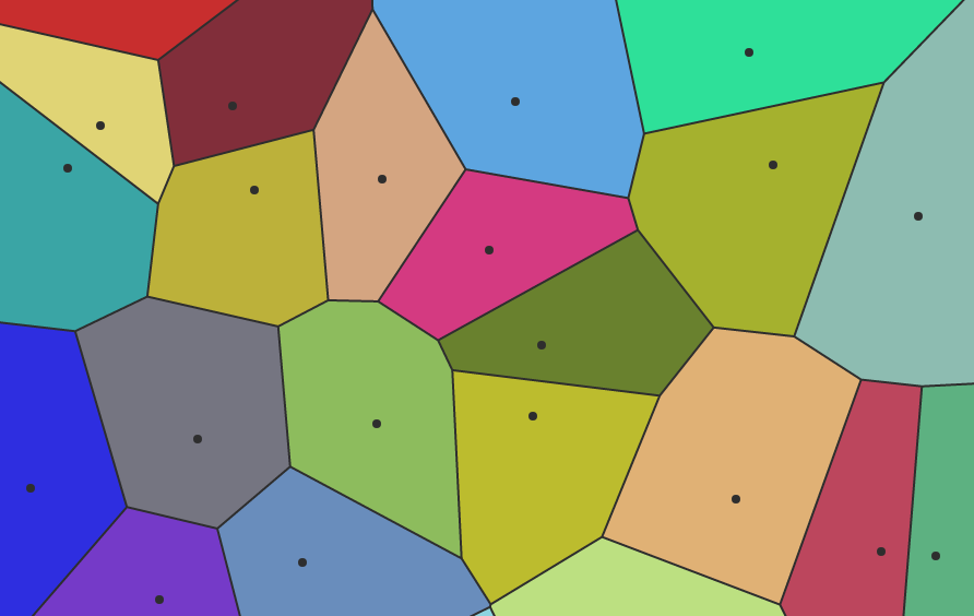
Voronoi cells. All images are by the author unless otherwise specified
In the previous article on Product Quantization for Similarity Search, we explained what product quantization is and went through in detail how product quantization works for similarity search.
Product quantization converts each vector in the database to a short code (PQ code), a representation that is intensely memory-efficient for the approximate nearest neighbor search.
As mentioned in the article, product quantization is highly scalable, but implementing product quantization alone is not the most effective method for large-scale searches.
In this post, we will examine and learn how product quantization can be integrated with the inverted file index to form a search method that is efficiently fast, and yet memory savvy.
IVFPQ is also commonly referred to as IVFADC in research papers.
Inverted File Index (IVF)
An inverted file is an index structure that is used to map contents to their locations.
You may probably ask, what are contents and locations, and how can the inverted file index apply to similarity search with product quantization?
Well, in our context, contents refer to the database vectors, and locations refer to the respective partitions where these vectors reside.
And yes, you heard it right, we need to partition the database vectors. The reason to partition the database vectors is so that search can be performed only on vectors of particular partitions, instead of all vectors.
Coarse Quantizer
First, the database vectors are separated into k' partitions. The partitioning is done through k-means clustering, producing what we called the coarse quantizer.
Here, an inverted file index is built, which will be used to map the list of vectors (i.e. inverted list) to the corresponding partition.

Each partition is represented and defined by a partition centroid, and each vector can only belong to one partition. This structure is sometimes referred to as the Voronoi cell, and hence search strategy based on partitions is also known as the cell-probe method_._

Example of Voronoi cells
Product Quantization on Residual Vectors
Next, for training and encoding, we employ the same process as described in Product Quantization for Similarity Search, except that this time the training and encoding are done on residual vectors instead of the original vectors.
What is Residual Vector
A residual vector is nothing but the offset of the vector from its partition centroid, i.e. the difference between the original vector and its associated partition centroid.
To compute the residual, we just subtract the centroid from the original vector.

Computing residual, the offset of the vector from its partition centroid
Why Residual Vectors
Why do we use residual vectors and go through the extra step of computing the residuals?
The intuition behind encoding the residual vector is to improve accuracy, as encoding the residual is more precise than encoding the original vector.
To understand what this means, we use a bunch of 3-dimensional vectors for illustration. Note that in real life, it is not practical to apply product quantization to such low-dimensional vectors. The 3-dimensional vectors are used here solely for explaining and visualizing them before and after computing the residuals.
In this example, the vectors can be distinctly segregated into two partitions, with the partition centroids denoted by red circles. There is also a query vector represented by an orange cross symbol. As illustrated below, this query vector is very close to Partition B.

First plot – Original vectors with two partitions
After computing the residual vectors, let’s see what they look like in the plot below.

Second plot – Residual vectors
First Observation
By taking the residuals, the data points from both partitions have virtually repositioned to the same space centered around the origin, and are overlapping with one another. This is very different from the first plot where the two partitions are seen to be isolated from one another.
Taking the residuals is akin to shifting the centroids to the origin, such that all data points are now focused on the origin.
Second Observation
Let’s pay attention to the query vector from the first plot and the residuals of the query vector from the second plot.
In the second plot, Query Residual A is the offset of the query vector from the centroid of Partition A, while Query Residual B is the offset of the query vector from the centroid of Partition B.
The distance of the query record to the respective partitions and data points remain the same before and after residual computation.
What can we conclude from all these observations?
It’s amazing that by taking the residuals, we managed to reduce the spread of the data points from all partitions and condense them to the same area while maintaining the same distance to the query record.
With a lower variance in the dataset, this would translate to smaller errors when doing the approximate nearest neighbor search using product quantization, and eventually result in better search quality.
Now, after understanding residual vectors and why they are being used, let’s get back to the product quantization process.
To recapitulate, a codebook is learned from the product quantization training, and PQ codes are generated from the encoding process.

The product quantization training and encoding process
With the presence of an inverted file index, the PQ codes are now included as part of the inverted list entry. As illustrated below, an entry for an inverted list would consist of the vector identifier (Vector Id) and the encoded residual (PQ code).

An inverted list entry consisting of Vector Id and PQ code
The entries are then added to the respective inverted lists tagged to the relevant partition.
Searching with IVFPQ
The coarse quantizer holds information on the list of partitions and the partition centroids. Given a query vector q, the coarse quantizer is used to find the partition centroid that is nearest to q.
After obtaining the partition centroid that is nearest to q, the residual of the query vector is computed.
Similar to the search procedure as described in Product Quantization for Similarity Search, we pre-calculate the partial squared Euclidean distance using the codebook and the residual of the query vector.
These partial squared Euclidean distances are recorded in a distance table with k rows and M columns, where M denotes the number of vector segments and k denotes the value selected to perform k-means clustering during training.
Now, with an inverted file index, we can selectively look up the partial distances and do a summation, only for those entries in the inverted list that are tagged to the partition where the partition centroid __ is nearest to q.
The inverted file index is the key component of a non-exhaustive search approach.
To find and return the
Knearest neighbors, one efficient way is to use a fixed capacity Max-Heap. This is a tree-based structure where the root node always contains the largest value, and each node would have a value that is equal to or smaller than the parent node.After each distance computation, the vector identifier is added to the Max-Heap structure only when its distance is smaller than the largest distance in the Max-Heap.
Improving Search Results
Earlier, with inverted file index, we talked about encoding residuals instead of original vectors to improve search results.
However, by searching only from one partition, we may encounter poorer results than that from a basic product quantization without an inverted file index.
While the search is incredibly fast with only one partition to probe, the result suffers because the search scope is now indeed limited to a very small subset of records.
According to the authors of Product Quantization for Nearest Neighbor Search [1],
"The query vector and its nearest neighbors are often not quantized to the same partition centroid, but to nearby ones"
As shown in the example below, although the query vector is nearest to the centroid at the partition on top, there are other vectors in nearby partitions that are also potential nearest neighbors of the query vector.

If the search is only confined to the partition where the query vector is nearest to that partition’s centroid, then we could miss out on many potential nearest neighbors that are residing at nearby partitions.
The effect is more apparent when the query vector is residing very near the border of a cell, or partition.
To avoid missing out on those potential nearest neighbors, a vector search can be performed on more partitions.
Particularly, we will perform a search on W partitions, where the centroids from these W partitions are nearest to the query vector. W is usually a parameter that is configurable.
What is the implication of having w > 1?
Well, with the inclusion of more partitions, we would need to compute the residual of the query vector separately with each partition centroid. And with each residual of the query vector, a separate distance table need to be computed.
Ultimately, the intention of performing a search on W partitions would result in computing W residual query vectors, and W distance tables.
Although there are overheads involved in building the inverted file index, for large datasets, having more partitions and searching from more partitions generally lead to better efficiency. This is the way to go and has proven to work very well in reality.
However, for small datasets, the complexity of the coarse quantizer may turn out to be the bottleneck if the number of partitions is too large.
Summary
The following diagram summarizes the processes and steps involved in similarity search with an inverted file index and product quantization (IVFPQ).

Similarity search with inverted file index and product quantization (IVFPQ)
With an inverted file index (IVF), a similarity search can be performed on pertinent partitions, confining the search scope to a small subset that is highly relevant.
On the other hand, product quantization (PQ) is capable of encoding vectors with a compressed representation that is extremely memory-efficient.
Implementing an inverted file index (IVF) with product quantization (PQ) institutes a novel method (IVFPQ) that is remarkably effective for large-scale similarity searches.
Putting the two together, we gain benefits from both worlds. The result? Fast search time with good accuracy for large-scale approximate nearest neighbor search.

Photo by James Baltz on Unsplash
P.S. Dealing with billion-sized vector datasets? Click the link below to learn about HNSW and how it can be used together with IVFPQ to form the best indexing approach for billion-scale similarity search.
References
[1] H. Jégou, M. Douze, C. Schmid, Product Quantization for Nearest Neighbor Search (2010)
[2] C. McCormick, Product Quantizers for k-NN Tutorial Part 2 (2017)
[3] J. Briggs, Product Quantization: Compressing high-dimensional vectors by 97%
Before You Go...Thank you for reading this post, and I hope you've enjoyed learning about similarity search with IVFPQ.If you like my post, don't forget to hit Follow and Subscribe to get notified via email when I publish.Optionally, you may also sign up for a Medium membership to get full access to every story on Medium.📑 Visit this GitHub repo for all codes and notebooks that I shared in my posts.© 2022 All rights reserved.Interested to read my other data science articles? Check out the following:
Transformers, can you rate the complexity of reading passages?
Advanced Techniques for Fine-tuning Transformers
Building a Product Recommendation Engine with AWS SageMaker