A Probabilistic Optimum-Path Forest Classifier for Non-Technical Losses Detection (original) (raw)
A Probabilistic Optimum-Path Forest Classifier for Non-Technical Losses Detection
Silas E. N. Fernandes, Danilo R. Pereira, Caio C. O. Ramos, André N. Souza, Danilo S. Gastaldello, João P. Papa
Abstract
Probabilistic-driven classification techniques extend the role of traditional approaches that output labels (usually integer numbers) only. Such techniques are more fruitful when dealing with problems where one is not interested in recognition/identification only, but also into monitoring the behavior of consumers and/or machines, for instance. Therefore, by means of probability estimates, one can take decisions to work better in a number of scenarios. In this paper, we propose a probabilisticbased Optimum-Path Forest (OPF) classifier to handle the problem of non-technical losses (NTL) detection in power distribution systems. The proposed approach is compared against naïve OPF, probabilistic Support Vector Machines, and Logistic Regression, showing promising results for both NTL identification and in the context of general-purpose applications.
Index Terms-Optimum-Path Forest, Probabilistic Classification, Non-technical Losses.
I. INTRODUCTION
PROBABILISTIC techniques play an important role in machine learning, since they extend the classification process to a greater range than simply labels. Very often we face problems where it is desirable to obtain some probability than just the label itself. Consider the problem of theft identification in energy distribution systems: electrical power companies consider much more fruitful to monitor the probability of a certain user to become a thief along the time instead of purely identifying such user. With the probabilities over time in hands, the company can take some preventive approach, which can be much more cost-effective than just punishing the user.
A seminal work conducted by Platt [1] extended the wellknown Support Vector Machines (SVM) to probabilistic classification. The idea is quite simple: to use SVMs’ outputs (labels) to feed a logistic function. Therefore, the initial outputs are mapped within the range [0,1][0,1]. However, in order to cope with problems related to different quantities (SVMs’ outputs before taking the signal to consider the final label), the author considered to use an optimization process over the whole training set in order to find out variables that regularize the label-probability mapping process. This technique is often referred to as “Platt Scaling”.
S. E. N. Fernandes was with the Department of Computing, Federal University of São Carlos, São Carlos, Brazil.
D. R. Pereira is with the University of Western São Paulo, Presidente Prudente, Brazil.
C. C. O. Ramos is with the Catarinense Federal Institute, Rio do Sul, Brazil
D. S. Gastaldello and A. N. Souza are with the Department of Electrical Engineering, São Paulo State University, Bauru, Brazil
J. P. Papa is with the Department of Computing, São Paulo State University, Bauru, Brazil.
Despite having a crucial role in the context of theft detection in power distribution systems, probabilistic-based approaches for non-technical losses (NTL) identification seem to not be the main focus of the related literature. As a matter of fact, most works rely on the detection of thefts using abstract-based machine learning algorithms. Ramos et al. [2]-[4] presented different approaches based on meta-heuristic techniques for firstly identifying the subset of features that describe better illegal consumers (i.e., characterization) for further recognizing them. Such approaches assume the problem of illegal consumer characterization can be modeled as a feature selection task. Recently, Leite and Mantovani [5] proposed an approach that performs detection and localization of illegal consumers in a single framework.
Non-technical losses detection is an issue often found in the so-called underdeveloped countries, and it mainly consists in the illegal tapping of distribution lines and tampering home meters. Also, NTL strongly affects the economy, since it influences the company’s revenues that could be applied to social programs and even enhancing the quality of the service provided by them. In a nutshell, non-technical losses refer to the amount of non-billed and billed electricity that is not paid for. Very recent works have also highlighted the importance of studies in such areas. Viegas et al. [6], for instance, surveyed a number of solutions that could be applied to cope with the problem of non-technical losses. The authors also pointed out that the main negative effects of NTL are commonly found in those countries with a fragile economy.
Other recent works also focused on the NTL problem. Han and Xiao [7] proposed a novel fraud detection for smart grids in the context of Colluded Non-Technical Losses, i.e., when many fraudsters act together to cheat the system. The proposed approach makes use of mathematical models that can identify multiple impostors. Lin et al. [8] considered the problem of NTL detection using non-cooperative games. In a nutshell, the main idea is to exploit previous consumption models and to use self-synchronization methods to learn the difference between those models and the real time meterreadings. Then, an approach based on non-cooperative games aims at identifying the abnormalities that are then correlated to the frauds.
Chatterjee et al. [9] employed the well-known Long-Short Term Memory networks to analyze the user’s consumption over time. The authors claim they can shortlist illegal consumers in real-time. Ahmad [10] considered low-voltage data from commercial, industrial, residential, and agricultural consumer to analyzed and inspected non-technical losses in Pakistan. The work presented a discussion concerning the
problem and how we can safeguard from further problems related to frauds in smart meters.
The work by Chatterjee et al. [9] considers an import aspect that is related to keep tracking users over time. Therefore, so essential as the identification of illegal consumers is their monitoring over time. By taking into account the identification framework only, one may recognize unlawful consumers only when their behavior is considerably far away from a normal one. In this context, the fraudster may be acting for a considerable time ago, which is quite money-taking regarding industrial consumers, for instance. However, probabilisticbased approaches produce soft outputs that can be analyzed and tracked over time. As an example, if the probabilities for a particular profile have increased considerably, we can decide to take precautions much earlier.
Some years ago, Papa et al. [11]-[13] introduced the supervised Optimum-Path Forest (OPF) classifier, which is a graphbased pattern recognition technique that uses a generalization of Dijkstra algorithm for multiple sources and path-cost functions. The OPF classifier has demonstrated interesting results in terms of efficiency and effectiveness, being some of them comparable to the ones obtained by SVMs, but usually faster for training, since OPF is parameterless and its training step has a quadratic complexity [11], [12]. As a matter of fact, Ramos et al. [14] and Passos et al. [15] were the first to evaluate the supervised [11], [12] and unsupervised versions [16] of the OPF classifier for NTL detection, respectively. Some years later, Trevisan et al. [17] combined Discrete Cosine Transform and the OPF classifier for automatic NTL identification. Later on, Guerrero et al. [18] combined artificial neural networks and text mining to reduce non-technical losses in power utilities.
However, the OPF classifier works with abstract (i.e., hard classification) outputs only. Also, as far as we know, there is only one very recent work that considered confidencebased OPF, but not for probability estimates [19], [20]. That work proposed to learn the confidence level (reliability) of each training sample when classifying others. Additionally, the cost-function used for conquering purposes was adapted to consider such reliability level. The authors showed the proposed confidence-based OPF works better in datasets with high concentration of overlapped samples. Therefore, to the best of our knowledge, there is no probabilistic-driven OPF to date, which turns to be the main contribution of this work. The proposed approach is evaluated in the context of generalpurpose problems and further for NTL identification in a private dataset obtained from a Brazilian power utility.
The remainder of this paper is organized as follows. Sections II and III present the OPF theoretical background and the probabilistic-driven approach, respectively. Section IV discusses the methodology and presents experiments. Finally, Section V states conclusions and future works.
II. OPTIMUM-PATH FOREST
The OPF framework is a recent highlight to the development of pattern recognition techniques based on graph partitions. The nodes are the data samples, which are represented by their corresponding feature vectors, and are connected according
to some predefined adjacency relation. Although the OPF classifier framework comprises supervised [11]-[13], semisupervised [21] and unsupervised versions [16], this work focused only on the supervised model, which is used to develop the proposed approach. Currently, there are two distinct versions of the OPF for supervised learning: (i) one that makes use of a complete graph [11], [12], and (ii) another version that uses a graph kk-neighborhood [11], [13], [22], [23].
The idea of the OPF classifier is to rule a competition process among some key samples (prototypes). Thus, the algorithm outputs an optimum path forest, which is a collection of optimum-path trees (OPTs) rooted at each prototype. Each OPT defines a discrete optimal partition (cluster) of samples that belong to the very same class, thus labelling the whole dataset with the label of each prototype sample. The next sections describe the OPF working mechanism in more details. This work employs the OPF classifier that use a complete graph, which is parameterless for training phase and is explained below.
A. Training phase
Let D=Dtr∪Dts\mathcal{D}=\mathcal{D}^{t r} \cup \mathcal{D}^{t s} be a λ\lambda-labeled dataset (i.e., λ\lambda stands for a function that can correctly label all dataset samples) such that Dtr\mathcal{D}^{t r} and Dts\mathcal{D}^{t s} stand for the training and testing sets, respectively. Additionally, let s∈D\mathbf{s} \in \mathcal{D} be an nn-dimensional sample that encodes features extracted from a certain data, and d(s,v)d(\mathbf{s}, \mathbf{v}) be a function that computes the distance between two samples s\mathbf{s} e v,v∈D\mathbf{v}, \mathbf{v} \in \mathcal{D}.
Let Gtr=(Dtr,A)\mathcal{G}^{t r}=\left(\mathcal{D}^{t r}, \mathcal{A}\right) be a graph derived from the training set, such that each node v∈Dtr\mathbf{v} \in \mathcal{D}^{t r} is connected to every other node in Dtr\v\mathcal{D}^{t r} \backslash \mathbf{v}, i.e. A\mathcal{A} defines an adjacency relation known as complete graph, in which the arcs are weighted by function d(⋅,⋅)d(\cdot, \cdot). We can also define a path πs\pi_{s} as a sequence of adjacent and distinct nodes in Gtr\mathcal{G}^{t r} with terminus at node s∈Dtr\mathbf{s} \in \mathcal{D}^{t r}. Notice a trivial path is denoted by ⟨s⟩\langle s\rangle, i.e. a single-node path.
Let f(πs)f\left(\pi_{s}\right) be a path-cost function that essentially assigns a real and positive value to a given path πs\pi_{s}, and S\mathcal{S} be a set of prototype nodes. Roughly speaking, OPF aims at minimizing f(πs)f\left(\pi_{\mathbf{s}}\right) for every sample in s∈Dtr\mathbf{s} \in \mathcal{D}^{t r}. The good point is that one does not need to deal with mathematical constraints, and the only rule to solve this problem concerns that all paths must be rooted at S\mathcal{S}. Therefore, we must choose two principles now: how to compute S\mathcal{S} (prototype estimation heuristic) and f(π)f(\pi) (path-cost function).
Since prototypes play a major role, Papa et al. [11] proposed to place them at the regions with the highest probabilities of misclassification, i.e. at the boundaries among samples from different classes. In fact, we are looking for the nearest samples from different classes, which can be computed by means of a Minimum Spanning Tree (MST) over Gtr\mathcal{G}^{t r}. The MST has interesting properties, which ensure OPF can be errorless during training when all arc-weights are different to each other [24].
Finally, with respect to the path-cost function, OPF requires ff to be a smooth one [11], [12], [25]. Previous experience in image segmentation led the authors to use a chain codeinvariant path-cost function, that basically computes the max-
imum arc-weight along a path, being denoted as fmaxf_{\max } and given by:
fmax(⟨s⟩)={0 if s∈S+∞ otherwise fmax(πs⋅(s,t))=max{fmax(πs),d(s,t)}\begin{aligned} f_{\max }(\langle s\rangle) & =\left\{\begin{array}{ll} 0 & \text { if } \mathbf{s} \in \mathcal{S} \\ +\infty & \text { otherwise } \end{array}\right. \\ f_{\max }\left(\pi_{s} \cdot(\mathbf{s}, \mathbf{t})\right) & =\max \left\{f_{\max }\left(\pi_{s}\right), d(\mathbf{s}, \mathbf{t})\right\} \end{aligned}
where πs⋅(s,t)\pi_{s} \cdot(\mathbf{s}, \mathbf{t}) stands for the concatenation between path πs\pi_{s} and arc(s,t)∈A\operatorname{arc}(\mathbf{s}, \mathbf{t}) \in \mathcal{A}, and d(s,t)d(\boldsymbol{s}, \boldsymbol{t}) stands for the distance between nodes s\boldsymbol{s} and t\boldsymbol{t}. Therefore, fmax(πs)f_{\max }\left(\pi_{\boldsymbol{s}}\right) computes the maximum distance among adjacent samples in πs\pi_{\boldsymbol{s}}, when πs\pi_{\boldsymbol{s}} is not a trivial path. In short, by computing fmaxf_{\max } for every sample s∈Dtr\mathbf{s} \in \mathcal{D}^{t r}, we obtain a collection of OPTs rooted at S\mathcal{S}, which then originate an optimum-path forest. A sample that belongs to a given OPT means it is more strongly connected to it than to any other in Gtr\mathcal{G}^{t r}. Roughly speaking, the OPF training step aims at solving Equation 1 in order to build the optimum-path forest. Figure 1 illustrates such training phase, and Algorithm 1 implements the above procedure for the OPF training phase [11], [12].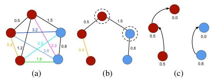
Fig. 1. Illustration of the OPF working mechanism: (a) a two-class (red and blue labels) training graph with weighted arcs, (b) an MST with prototypes highlighted, and © optimum-path forest generated during the training phase with costs over the nodes (notice the prototypes have zero cost).
Lines 1−41-4 initialize maps and insert prototypes in QQ (the function λ(⋅)\lambda(\cdot) in Line 4 assigns the true label to each training sample) 1{ }^{1}. The main loop computes an optimum path from S\mathcal{S} to every sample s\boldsymbol{s} in a non-decreasing order of cost (Lines 5−145-14 ). At each iteration, a path of minimum cost CsC_{\boldsymbol{s}} is obtained in PP when we remove its last node s\boldsymbol{s} from QQ (Line 6). Ties are broken in QQ using first-in-first-out policy. That is, when two optimum paths reach an ambiguous sample s\boldsymbol{s} with the same minimum cost, s\boldsymbol{s} is assigned to the first path that reached it. Note that Ct>CsC_{\boldsymbol{t}}>C_{\boldsymbol{s}} in Line 8 is false when t\boldsymbol{t} has been removed from QQ and, therefore, Ct≠+∞C_{\boldsymbol{t}} \neq+\infty in Line 11 is true only when t∈Q\boldsymbol{t} \in Q. Lines 10−1410-14 evaluate whether the path that reaches an adjacent node t\boldsymbol{t} through s\boldsymbol{s} is cheaper than the current path with terminus t\boldsymbol{t}, and update the position of t\boldsymbol{t} in Q,Ct,LtQ, C_{\boldsymbol{t}}, L_{\boldsymbol{t}} and PtP_{\boldsymbol{t}} accordingly.
B. Classification phase
The next step concerns the testing phase, where each sample t∈Dts\mathbf{t} \in \mathcal{D}^{t s} is classified individually as follows: t\mathbf{t} is connected to all training nodes from the optimum-path forest learned in the training phase (Figure 2a), and it is evaluated the node v∗∈Dtr\mathbf{v}^{*} \in \mathcal{D}^{t r} that conquers t\mathbf{t}, which is basically to evaluate the optimum cost CtC_{\boldsymbol{t}} as follows [11], [12]:
[1]Algorithm 1: Optimum-Path Forest Training Algorithm
Input: A labeled training set Dtr\mathcal{D}^{t r}.
Output: Optimum-path forest PP, cost map CC, label map LL, and ordered set D^tr\hat{D}^{t r}.
Auxiliary: Priority queue QQ, set S\mathcal{S} of prototypes, and cost variable cst.
1 Set D^tr←∅\hat{D}^{t r} \leftarrow \emptyset and compute the set of prototypes S⊂Dtr\mathcal{S} \subset \mathcal{D}^{t r} by MST ;
2 For each s∈Dtr\S\boldsymbol{s} \in \mathcal{D}^{t r} \backslash \mathcal{S}, set Cs←+∞C_{\boldsymbol{s}} \leftarrow+\infty;
3 for each s∈S\boldsymbol{s} \in \mathcal{S} do
4Cs←0,Ps←nil,Ls←λ(s)4 C_{\boldsymbol{s}} \leftarrow 0, P_{\boldsymbol{s}} \leftarrow n i l, L_{\boldsymbol{s}} \leftarrow \lambda(\boldsymbol{s}), and insert s\boldsymbol{s} in QQ;
5 while QQ is not empty do
6 Remove from QQ a sample s\boldsymbol{s} such that CsC_{\boldsymbol{s}} is minimum;
7 Insert s\boldsymbol{s} in D^tr\hat{D}^{t r};
8 for each t∈Dtr\boldsymbol{t} \in \mathcal{D}^{t r} such that Ct>CsC_{\boldsymbol{t}}>C_{\boldsymbol{s}} do
9 Compute cst←max{Cs,d(s,t)}\operatorname{cst} \leftarrow \max \left\{C_{\boldsymbol{s}}, d(\boldsymbol{s}, \boldsymbol{t})\right\};
10 if cst<Ctc s t<C_{\boldsymbol{t}} then
11 if Ct≠+∞C_{\boldsymbol{t}} \neq+\infty then
12 Remove t\boldsymbol{t} from QQ;
13
Pt←s,Lt←Ls,Ct←cst;P_{\boldsymbol{t}} \leftarrow \boldsymbol{s}, L_{\boldsymbol{t}} \leftarrow L_{\boldsymbol{s}}, C_{\boldsymbol{t}} \leftarrow \operatorname{cst} ;
14 Insert t\boldsymbol{t} in QQ;
15 return [P,C,L,D^tr]\left[P, C, L, \hat{D}^{t r}\right]
Ct=argminv∈Dtr{max{Cv,d(v,t)}}C_{\mathbf{t}}=\underset{\mathbf{v} \in \mathcal{D}^{t r}}{\arg \min }\left\{\max \left\{C_{\mathbf{v}}, d(\mathbf{v}, \mathbf{t})\right\}\right\}
Let the node v∗∈Dtr\mathbf{v}^{*} \in \mathcal{D}^{t r} be the one that satisfies Equation 2. The classification step simply assigns the label t=λ(v∗)\mathbf{t}=\lambda\left(\mathbf{v}^{*}\right), as depicted in Figure 2b, where λ(v∗)\lambda\left(\mathbf{v}^{*}\right) stands for the true label of sample v∗\mathbf{v}^{*}. Roughly speaking, the testing step aims at finding the training node v\mathbf{v} that minimizes CtC_{\mathbf{t}}.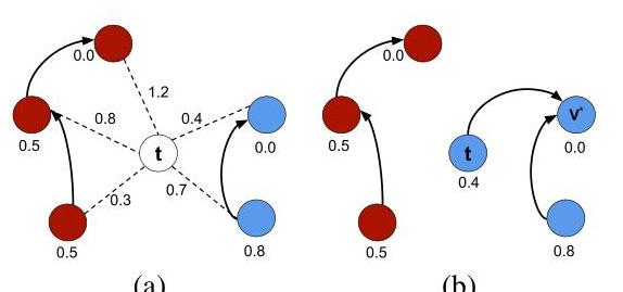
Fig. 2. Illustration of the OPF classification mechanism: (a) sample t\mathbf{t} is connected to all training nodes, and (b) t\mathbf{t} is conquered by v∗\mathbf{v}^{*}, and it receives the “blue” label.
Algorithm 2 implements the OPF classification procedure [11], [12]. The main loop (Lines 1−81-8 ) performs the classification of all nodes in Dts\mathcal{D}^{t s}. The inner loop (Lines 3−83-8 ) visits each node ki+1∈D‾tr,i=1,2,⋯ ,∣D1r∣−1\boldsymbol{k}_{i+1} \in \overline{\mathcal{D}}^{t r}, i=1,2, \cdots,\left|\mathcal{D}_{1}^{r}\right|-1 until an optimum path πki+1⋅⟨ki+1,t⟩\pi_{\boldsymbol{k}_{i+1}} \cdot\left\langle\boldsymbol{k}_{i+1}, \boldsymbol{t}\right\rangle is found. In the worst case, the algorithm visits all nodes in D‾tr\overline{\mathcal{D}}^{t r}. Line 4 evaluates fmax(πki+1⋅⟨ki+1,t⟩)f_{\max }\left(\pi_{\boldsymbol{k}_{i+1}} \cdot\left\langle\boldsymbol{k}_{i+1}, \boldsymbol{t}\right\rangle\right) and Lines 6−76-7 update the cost, label and predecessor of t\boldsymbol{t}.
- 1{ }^{1} The cost map CC stores the optimum-cost of each training sample. ↩︎
Algorithm 2: Optimum-Path Forest Classification Algorithm.
Input: Classifier [P,C,L,Dtr^]\left[P, C, L, \widehat{\mathcal{D}^{t r}}\right] and a test set Dts\mathcal{D}^{t s}.
Output: Label L′L^{\prime}, cost C′C^{\prime} and predecessor P′P^{\prime} maps defined for Dts\mathcal{D}^{t s}.
Auxiliary: Cost variables tmp and mincost.
for each \(\boldsymbol{t} \in \mathcal{D}^{t s}\) do
    \(i \leftarrow 0\), mincost \(\leftarrow \max \left\{C_{\boldsymbol{k}_{i}}, d\left(\boldsymbol{k}_{i}, \boldsymbol{t}\right)\right\} L_{\boldsymbol{t}}^{\prime} \leftarrow L_{\boldsymbol{k}_{i}}\)
        \(P_{\boldsymbol{t}}^{\prime} \leftarrow \boldsymbol{k}_{i}\) and \(C_{\boldsymbol{t}}^{\prime} \leftarrow\) mincost;
    while \(i<\left|\mathcal{D}^{t r}\right|\) and mincost \(>C_{\boldsymbol{k}_{i+1}}\) do
        Compute tmp \(\leftarrow \max \left\{C_{\boldsymbol{k}_{i+1}}, d\left(\boldsymbol{k}_{i+1}, \boldsymbol{t}\right)\right\}\);
        if tmp \(<\) mincost then
            mincost \(\leftarrow\) tmp and \(C_{\boldsymbol{t}}^{\prime} \leftarrow\) mincost;
            \(L_{\boldsymbol{t}}^{\prime} \leftarrow L_{\boldsymbol{k}_{i+1}}\) and \(P_{\boldsymbol{t}}^{\prime} \leftarrow \boldsymbol{k}_{i+1}\);
    \(i \leftarrow i+1\);
9 return \(\left[L^{\prime}, C^{\prime}, P^{\prime}\right]\)
III. Probabilistic Optimum-Path Forest
The probabilistic OPF is inspired in the Platt Scaling approach, which basically ends up mapping the SVMs’ output to probability estimates. Therefore, before introducing the proposed approach, one must master the Platt Scaling mechanism.
A. Probabilistic Support Vector Machines
Considering the labeled dataset D\mathcal{D} described in Section II, let us assume each sample xi∈D\mathbf{x}_{i} \in \mathcal{D} can be assigned to a class label yi∈{−1,+1},i=1,2,…,∣D∣y_{i} \in\{-1,+1\}, i=1,2, \ldots,|\mathcal{D}|. Platt proposed to approximate the posterior class probability P(yi=1∣xi)P\left(y_{i}=1 \mid \mathbf{x}_{i}\right) as follows [1]:
P(yi=1∣xi)≈PA,B(fi)=11+exp(Afi+B)P\left(y_{i}=1 \mid \mathbf{x}_{i}\right) \approx P_{A, B}\left(f_{i}\right)=\frac{1}{1+\exp \left(A f_{i}+B\right)}
where fif_{i} stands for the output (decision function) of SVMs concerning sample xi\mathbf{x}_{i}. Let θ=(A∗,B∗)\theta=\left(A^{*}, B^{*}\right) be the best set of parameters that can be determined by the following maximum likelihood problem:
argminθF(θ)=−∑i=1m(yilog(pi)+(1−yi)log(1−pi))\underset{\theta}{\arg \min } F(\theta)=-\sum_{i=1}^{m}\left(y_{i} \log \left(p_{i}\right)+\left(1-y_{i}\right) \log \left(1-p_{i}\right)\right)
where pi=PA,B(fi)p_{i}=P_{A, B}\left(f_{i}\right) and mm denotes the number of samples to be considered. Essentially, the above equation stands for the cost function of the well-known Logistic Regression classifier.
In order to avoid overfitting, Platt proposed to regularize Equation 4 as follows:
argminθF(θ)=−∑i=1m(tilog(pi)+(1−ti)log(1−pi))\underset{\theta}{\arg \min } F(\theta)=-\sum_{i=1}^{m}\left(t_{i} \log \left(p_{i}\right)+\left(1-t_{i}\right) \log \left(1-p_{i}\right)\right)
where tit_{i} is formulated as follows:
ti={N++1N++2 if yi=+11N−+2 if yi=−1t_{i}= \begin{cases}\frac{N_{+}+1}{N_{+}+2} & \text { if } y_{i}=+1 \\ \frac{1}{N_{-}+2} & \text { if } y_{i}=-1\end{cases}
In the above formulation, N+N_{+}N+and N−N_{-}N−stand for the number of positive and negative samples, respectively. In short, tit_{i} can be used to handle unbalanced datasets as well.
B. Modified Probabilistic Support Vector Machines
Almost a decade later the seminal work of Platt, Lin et al. [26] highlighted some numerical instabilities related to Equation 5:
- we know that log\log and exp\exp functions can easily cause an overflow, since exp(Afi+B)→∞\exp \left(A f_{i}+B\right) \rightarrow \infty when Afi+BA f_{i}+B is large enough. Additionally, log(pi)→−∞\log \left(p_{i}\right) \rightarrow-\infty when pi→0p_{i} \rightarrow 0.
- according to Goldberg [27], 1−pi=1−11+exp(Afi+B)1-p_{i}=1-\frac{1}{1+\exp \left(A f_{i}+B\right)} is a “catastrophic cancellation” when pip_{i} is close to one. Such term arises from the fact we need to subtract two relatively close number that are already results of previous floating-point operations. Lin et al. [26] described an interesting example: suppose fi=1f_{i}=1 and (A,B)=(−64,0)(A, B)=(-64,0). In this case, 1−pi1-p_{i} returns 0 , but its equivalent formulation exp(Afi+B)1+exp(Afi+B)\frac{\exp \left(A f_{i}+B\right)}{1+\exp \left(A f_{i}+B\right)} gives a more accurate result. Also, the very same group of authors stated the aforementioned catastrophic cancellation induces most of the log(0)\log (0) occurrences.
In order to deal with the aforementioned situation, Lin et al. [26] proposed to reformulate the cost function F(θ)F(\theta) as follows:
F(θ)=−∑i=1m(tilog(pi)+(1−ti)log(1−pi))=∑i=1m((ti−1)(qi)+log(1+exp(qi)))=∑i=1m(tiqi+log(1+exp(−Afi−B)))\begin{aligned} F(\theta) & =-\sum_{i=1}^{m}\left(t_{i} \log \left(p_{i}\right)+\left(1-t_{i}\right) \log \left(1-p_{i}\right)\right) \\ & =\sum_{i=1}^{m}\left(\left(t_{i}-1\right)\left(q_{i}\right)+\log \left(1+\exp \left(q_{i}\right)\right)\right) \\ & =\sum_{i=1}^{m}\left(t_{i} q_{i}+\log \left(1+\exp \left(-A f_{i}-B\right)\right)\right) \end{aligned}
where qi=Afi+Bq_{i}=A f_{i}+B. Therefore, considering the above formulation, 1−pi1-p_{i} and log(0)\log (0) do not happen 2{ }^{2}.
However, even if using Equations 8 and 9, the overflow problem may still occur. In order to cope with such problem, Lin et al. [26] proposed to apply Equation 9 when Afi+B≥A f_{i}+B \geq 0 ; otherwise, one should use Equation 8.
C. Proposed Approach for Probabilistic Outputs
In this section, we present the theoretical background concerning the Probabilistic Optimum-Path Forest (P-OPF). Since the cost assigned to each sample during training and classification with OPF is positive (Equation 2), we need some minor adjustments with respect to Equation 3, which can be rewritten to accommodate OPF requirements:
P(y^i=yi∣xi)≈PA,B(Ci)=11+exp(AyiCi+B)P\left(\hat{y}_{i}=y_{i} \mid \mathbf{x}_{i}\right) \approx P_{A, B}\left(C_{i}\right)=\frac{1}{1+\exp \left(A y_{i} C_{i}+B\right)}
where CiC_{i} stands for the cost assigned to sample xi\mathbf{x}_{i} during OPF training or classification step, and yi^\hat{y_{i}} denotes the label
- 2{ }^{2} Please, consider taking a look at the work of Lin et al. [26] for a more detailed explanation of the mathematical formulation. ↩︎
predicted by the classifier. Basically, we ended up replacing fif_{i} by yiCiy_{i} C_{i}, since the cost function CiC_{i} is not signed, while sgn(fi)∈{−,+}\operatorname{sgn}\left(f_{i}\right) \in\{-,+\}. The rationale behind the proposed approach is to assume the lower the cost assigned to sample xi\mathbf{x}_{i}, i.e. CiC_{i}, the higher the probability of that sample be correctly classified.
The cost function F(θ)F(\theta) needs to be reformulated to consider P-OPF model, as follows:
F(θ)=−∑i=1m(tilog(pi)+(1−ti)log(1−pi))=∑i=1m((ti−1)(qi)+log(1+exp(qi)))=∑i=1m(tiqi+log(1+exp(−AyiCi−B)))\begin{aligned} F(\theta) & =-\sum_{i=1}^{m}\left(t_{i} \log \left(p_{i}\right)+\left(1-t_{i}\right) \log \left(1-p_{i}\right)\right) \\ & =\sum_{i=1}^{m}\left(\left(t_{i}-1\right)\left(q_{i}\right)+\log \left(1+\exp \left(q_{i}\right)\right)\right) \\ & =\sum_{i=1}^{m}\left(t_{i} q_{i}+\log \left(1+\exp \left(-A y_{i} C_{i}-B\right)\right)\right) \end{aligned}
where pi=PA,B(Ci)p_{i}=P_{A, B}\left(C_{i}\right). Last but not least, one must use the trick proposed by Lin et al. [26], i.e., if AyiCi+B≥0A y_{i} C_{i}+B \geq 0, then one shall use
exp(−AyiCi−B)1+exp(−AyiCi−B)\frac{\exp \left(-A y_{i} C_{i}-B\right)}{1+\exp \left(-A y_{i} C_{i}-B\right)}
otherwise one shall use
11+exp(AyiCi+B)\frac{1}{1+\exp \left(A y_{i} C_{i}+B\right)}
After learning parameters AA and BB, we then compute the probability of each sample to belong to class +1 , i.e. P(y^i=1∣xi)P\left(\hat{y}_{i}=1 \mid \mathbf{x}_{i}\right). If P(y^i=1∣xi)>P(y^i=0∣xi)P\left(\hat{y}_{i}=1 \mid \mathbf{x}_{i}\right)>P\left(\hat{y}_{i}=0 \mid \mathbf{x}_{i}\right), then P-OPF assigns the label +1 to that sample; otherwise the sample is assigned to class -1 . In this work, we adopted Θ=0.5\Theta=0.5, since it models a single chance. However, one can easily fine-tune that threshold using a linear-search or any other optimization algorithm. Algorithm 3 implements the probabilistic OPF classifier.
Line 1 executes the OPF training algorithm presented in Section II-A, and it outputs the label, cost and predecessor maps, as well as the ordered set of training samples by the cost map. Line 2 classifies the validating set according to the procedure described in Section II-B, and the loop in Lines 12−2512-25 are in charge of optimizing parameters AA and BB, i.e., they aim at computing the best set of parameters θ\theta using a grid search over the ranges A∈[LA,UA]A \in\left[L_{A}, U_{A}\right] and B∈[LB,UB]B \in\left[L_{B}, U_{B}\right], where LAL_{A} and UAU_{A} stand for the lower and upper bounds considering parameter AA. The same can be defined for variable BB. Finally, Line 26 stores the best set of parameters θ\theta, which are then used to compute the probability of each test sample in Lines 27−3127-31.
IV. DATA AND EXPERIMENTAL DESIGN
In this section, we present the methodology and experiments employed to validate the effectiveness and efficiency of the proposed approach. Firstly, in Section IV-A, we validate the effectiveness of P-OPF against standard OPF in some benchmark problems. Further, in Section IV-B, we compare the proposed approach in the context of NTL identification.
Algorithm 3: Probabilistic Optimum-Path Forest Al-
gorithm
Input: A λ\lambda-labeled training Gtr=(Dtr,A)\mathcal{G}^{t r}=\left(\mathcal{D}^{t r}, \mathcal{A}\right) and validating Gvl=(Dvl,A)\mathcal{G}^{v l}=\left(\mathcal{D}^{v l}, \mathcal{A}\right) sets, unlabeled test Gts=(Dts,A)\mathcal{G}^{t s}=\left(\mathcal{D}^{t s}, \mathcal{A}\right) set, and the ranges [LA,UA]\left[L_{A}, U_{A}\right] and [LB,UB]\left[L_{B}, U_{B}\right] concerning parameters AA and BB, respectively.
Output: Probability output for each sample in Dts\mathcal{D}^{t s}.
1[P,C,L,D^tr]←1\left[P, C, L, \hat{\mathcal{D}}^{t} r\right] \leftarrow Algorithm 1(Dtr)1\left(\mathcal{D}^{t r}\right);
2[P′,C′,L′]←2\left[P^{\prime}, C^{\prime}, L^{\prime}\right] \leftarrow Algorithm 2([P,C,L,D^tr],Dvl)2\left(\left[P, C, L, \hat{\mathcal{D}}^{t} r\right], \mathcal{D}^{v l}\right);
3N+←03 N_{+} \leftarrow 0 and N−←0N_{-} \leftarrow 0;
4 for each v∈Dvl\boldsymbol{v} \in \mathcal{D}^{v l} do
5 if λ(v)=+1\lambda(\boldsymbol{v})=+1 then
6N+←N++1;6 \quad N_{+} \leftarrow N_{+}+1 ;
7 else
8N−←N−+1;8 \quad N_{-} \leftarrow N_{-}+1 ;
9t+←N++1N++2;9 t_{+} \leftarrow \frac{N_{+}+1}{N_{+}+2} ;
10t−←1N−+2;10 t_{-} \leftarrow \frac{1}{N_{-}+2} ;
11A∗←0,B∗←0,min F←+∞;11 A^{*} \leftarrow 0, B^{*} \leftarrow 0, \min \mathrm{~F} \leftarrow+\infty ;
12 for each Ai∈[LA,UA],Bj∈[LB,UB]A_{i} \in\left[L_{A}, U_{A}\right], B_{j} \in\left[L_{B}, U_{B}\right] do
for each v∈Dvl\boldsymbol{v} \in \mathcal{D}^{v l} do
if λ(v)=+1\lambda(\boldsymbol{v})=+1 then
t←t+t \leftarrow t_{+};
else
t←t−;t \leftarrow t_{-} ;
if AiCv+Bj≥0A_{i} C_{\mathbf{v}}+B_{j} \geq 0 then
Fij←Fij+(t(Aiλ(v)Cv+Bj)+F_{i j} \leftarrow F_{i j}+\left(t\left(A_{i} \lambda(\mathbf{v}) C_{\mathbf{v}}+B_{j}\right)+\right.
log(1+exp(−Aiλ(v)Cv−Bj)))\left.\log \left(1+\exp \left(-A_{i} \lambda(\mathbf{v}) C_{\mathbf{v}}-B_{j}\right)\right)\right) ;
else
Fij←Fij+(t−1)∗(Aiλ(v)Cv+Bj)+F_{i j} \leftarrow F_{i j}+(t-1) *\left(A_{i} \lambda(\mathbf{v}) C_{\mathbf{v}}+B_{j}\right)+
log(1+exp(Aiλ(v)Cv+Bj));\log \left(1+\exp \left(A_{i} \lambda(\mathbf{v}) C_{\mathbf{v}}+B_{j}\right)\right) ;
if Fij<minFF_{i j}<\min F then
min{i←Ai;\min \left\{{ }_{i} \leftarrow A_{i} ;\right.
B∗←Bj;B^{*} \leftarrow B_{j} ;
26θ←(A∗,B∗);26 \theta \leftarrow\left(A^{*}, B^{*}\right) ;
27 for each i∈Dts\boldsymbol{i} \in \mathcal{D}^{t s} do
if (A∗λ(i)Ci+B∗)≥0\left(A^{*} \lambda(\boldsymbol{i}) C_{\boldsymbol{i}}+B^{*}\right) \geq 0 then
Pi←exp(−A∗λ(i)Ci−B∗)1+exp(−A∗λ(i)Ci−B∗)P_{\mathbf{i}} \leftarrow \frac{\exp \left(-A^{*} \lambda(\mathbf{i}) C_{\mathbf{i}}-B^{*}\right)}{1+\exp \left(-A^{*} \lambda(\mathbf{i}) C_{\mathbf{i}}-B^{*}\right)};
else
Pi←11+exp(A∗λ(i)Ci+B∗);P_{\mathbf{i}} \leftarrow \frac{1}{1+\exp \left(A^{*} \lambda(\mathbf{i}) C_{\mathbf{i}}+B^{*}\right)} ;
A. Experiments over General-purpose Datasets
In order to fine-tune parameters AA and BB, we employed two different strategies, being one of them based on metaheuristics, and another one purely mathematical. In regard to the meta-heuristic-driven techniques, we opted to use Particle Swarm Optimization (PSO) [28], hereinafter denoted as P-OPF-PSO, and with respect to the mathematical approach we used the well-known Newton method with Backtracking line
search for solving Equation 4, hereinafter denoted as P-OPFNB, as described by Lin et al. [26]. To study the behavior of P-OPF under different scenarios, we used two synthetic (synhetic01, synhetic02) and nine public benchmarking datasets 3{ }^{3}. These datasets have been frequently used in the evaluation of different classification methods. The datasets were normalized as follows:
t′=t−μρ\mathbf{t}^{\prime}=\frac{\mathbf{t}-\mu}{\rho}
where μ\mu denotes the mean, and ρ\rho stands for its standard deviation. Also, tt and t′t^{\prime} correspond to the original and normalized features, respectively. Table I presents the main characteristics of each dataset.
TABLE I
INFORMATION ABOUT THE BENCHMARKING DATASETS USED IN THIS WORK.
| Dataset | No. of samples | No. of features | No. of classes |
|---|---|---|---|
| UCI-Adult | 32,561 | 123 | 2 |
| Statlog-Australian | 690 | 14 | 2 |
| Pima-Indians-Diabetes | 768 | 8 | 2 |
| UCI-Ionosphere | 351 | 34 | 2 |
| UCI-Lexkemia | 72 | 7,129 | 2 |
| UCI-Liver-disorders | 345 | 6 | 2 |
| UCI-Madelon | 2,600 | 500 | 2 |
| UCI-Sonar | 208 | 60 | 2 |
| UCI-Splice | 3,175 | 60 | 2 |
| Synthetic01 | 1,000 | 2 | 2 |
| Synthetic02 | 1,000 | 2 | 2 |
Regarding the methodology, each dataset was partitioned into three subsets, training ( 40%40 \% ), validating ( 20%20 \% ) and testing sets ( 40%40 \% ), hereinafter denoted as 40:20:4040: 20: 40. For each range, training, validating, and testing sets were selected randomly and the process was repeated 30 times (cross-validation) 4{ }^{4} It is worth noting the standard OPF was trained over Dtr∪Dvl\mathcal{D}^{t r} \cup \mathcal{D}^{v l} considering the aforementioned three stages. After learning, P-OPF-PSO and P-OPF-NB were trained once more using the original training set (i.e., the very same one used by OPF). In order to compare the proposed approach, we computed the mean accuracy and execution time for the further usage of the Wilcoxon signed rank test [29] with significance of 0.05 .
Regarding the optimization techniques, we used 500 agents (initial solutions) concerning PSO, c1=1.4,c2=0.6,w=0.5c_{1}=1.4, c_{2}=0.6, w=0.5, as well as 100 iterations for convergence. Variables c1c_{1} and c2c_{2} are used to weight the importance of a possible solution being far or close to the local and global optimum, respectively. Variable ww stands for the well-known “inertia weight”, which is used as a step size towards better solutions. The search space for A×BA \times B was defined within [−5,5]×[−5,5][-5,5] \times[-5,5]. Once again, these values have been empirically chosen. With respect to the Newton method, we used a maximum number of iterations of 1000 , minimum step in the linear search of 1e−121 e-12 and σ=1e−12\sigma=1 e-12.
Table II presents the mean accuracies and standard deviation over all datasets, being the recognition rates computed
[1]according to Papa et al. [11], and Table III presents the mean F-measure values concerning the very same group of datasets. The most accurate techniques considering the Wilcoxon test are highlighted in bold. As one can observe, both P-OPFPSO and standard OPF showed close results in almost all datasets, except “UCI-Adult”, which is better generalized by P-OPF using PSO, and “UCI-Liver-disorders”, which is better generalized by standard OPF.
TABLE II
MEAN ACCURACY RESULTS CONSIDERING STANDARD OPF, P-OPF AND ITS VARIATIONS UNDER DIFFERENT OPTIMIZATION TECHNIQUES.
| Dataset | P-OPF-NB | P-OPF-PSO | OPF |
|---|---|---|---|
| UCI-Adult | 61.87±2.1361.87 \pm 2.13 | 67.42±1.02\mathbf{6 7 . 4 2} \pm 1.02 | 65.42±1.1465.42 \pm 1.14 |
| Statlog-Australian | 78.54±1.97\mathbf{7 8 . 5 4} \pm 1.97 | 78.35±2.0078.35 \pm 2.00 | 78.35±2.0078.35 \pm 2.00 |
| Pima-Indians-Diabetes | 65.41±2.44\mathbf{6 5 . 4 1} \pm 2.44 | 63.36±8.01\mathbf{6 3 . 3 6} \pm 8.01 | 65.39±2.41\mathbf{6 5 . 3 9} \pm 2.41 |
| UCI-Ionosphere | 78.88±3.7878.88 \pm 3.78 | 78.57±12.04\mathbf{7 8 . 5 7} \pm 12.04 | 80.78±3.68\mathbf{8 0 . 7 8} \pm 3.68 |
| UCI-Lexkemia | 79.35±7.84\mathbf{7 9 . 3 5} \pm 7.84 | 75.73±16.14\mathbf{7 5 . 7 3} \pm 16.14 | 79.35±7.84\mathbf{7 9 . 3 5} \pm 7.84 |
| UCI-Liver-disorders | 60.37±4.7060.37 \pm 4.70 | 60.13±4.9060.13 \pm 4.90 | 60.96±4.60\mathbf{6 0 . 9 6} \pm 4.60 |
| UCI-Madelon | 52.72±1.38\mathbf{5 2 . 7 2} \pm 1.38 | 52.72±1.38\mathbf{5 2 . 7 2} \pm 1.38 | 52.72±1.38\mathbf{5 2 . 7 2} \pm 1.38 |
| UCI-Sonar | 82.21±4.33\mathbf{8 2 . 2 1} \pm 4.33 | 82.21±4.33\mathbf{8 2 . 2 1} \pm 4.33 | 82.21±4.33\mathbf{8 2 . 2 1} \pm 4.33 |
| UCI-Splice | 54.09±1.7854.09 \pm 1.78 | 55.99±1.63\mathbf{5 5 . 9 9} \pm 1.63 | 54.42±1.5654.42 \pm 1.56 |
| Synthetic01 | 60.52±1.8260.52 \pm 1.82 | 60.99±1.82\mathbf{6 0 . 9 9} \pm 1.82 | 60.99±1.82\mathbf{6 0 . 9 9} \pm 1.82 |
| Synthetic02 | 89.50±1.8089.50 \pm 1.80 | 90.20±1.54\mathbf{9 0 . 2 0} \pm 1.54 | 90.20±1.54\mathbf{9 0 . 2 0} \pm 1.54 |
The FF-measure statistical analysis showed a similar behavior to the ones obtained by standard accuracy, as it can be observed in Table III. Both P-OPF and standard OPF showed close results in 8 out of 11 datasets concerning the the accuracy results. Only “UCI-Liver-disorders” dataste can be better generalized by standard OPF. Furthermore, “UCI-Adult” dataset showed a similar result for both P-OPF-PSO and standard OPF regarding the F-measure. In general, P-OPF using PSO was more effective for finding the best set of parameters. Although P-OPF and standard OPF achieved similar results according to accuracy and FF-measure, it is worth noting that the P-OPF was able to encode output probability estimates. This idea can be promising in several cases, such as in multiple classifiers that use confidence-oriented techniques instead of abstract outputs.
TABLE III
MEAN FF-MEASURE VALUES.
| Dataset | P-OPF-NB | P-OPF-PSO | OPF |
|---|---|---|---|
| UCI-Adult | 0.6134±0.01480.6134 \pm 0.0148 | 0.6384±0.0122\mathbf{0 . 6 3 8 4} \pm 0.0122 | 0.6384±0.0132\mathbf{0 . 6 3 8 4} \pm 0.0132 |
| Statlog-Australian | 0.7860±0.0194\mathbf{0 . 7 8 6 0} \pm 0.0194 | 0.7840±0.01960.7840 \pm 0.0196 | 0.7840±0.01960.7840 \pm 0.0196 |
| Pima-Indians-Diabetes | 0.6544±0.0233\mathbf{0 . 6 5 4 4} \pm 0.0233 | 0.6311±0.0896\mathbf{0 . 6 3 1 1} \pm 0.0896 | 0.6542±0.0230\mathbf{0 . 6 5 4 2} \pm 0.0230 |
| UCI-Ionosphere | 0.8078±0.03800.8078 \pm 0.0380 | 0.8013±0.1317\mathbf{0 . 8 0 1 3} \pm 0.1317 | 0.8257±0.0361\mathbf{0 . 8 2 5 7} \pm 0.0361 |
| UCI-Lexkemia | 0.8009±0.0780\mathbf{0 . 8 0 0 9} \pm 0.0780 | 0.7621±0.1734\mathbf{0 . 7 6 2 1} \pm 0.1734 | 0.8009±0.0780\mathbf{0 . 8 0 0 9} \pm 0.0780 |
| UCI-Liver-disorders | 0.6034±0.04760.6034 \pm 0.0476 | 0.6010±0.04960.6010 \pm 0.0496 | 0.6093±0.0467\mathbf{0 . 6 0 9 3} \pm 0.0467 |
| UCI-Madelon | 0.5252±0.0138\mathbf{0 . 5 2 5 2} \pm 0.0138 | 0.5252±0.0138\mathbf{0 . 5 2 5 2} \pm 0.0138 | 0.5252±0.0138\mathbf{0 . 5 2 5 2} \pm 0.0138 |
| UCI-Sonar | 0.8235±0.0437\mathbf{0 . 8 2 3 5} \pm 0.0437 | 0.8235±0.0437\mathbf{0 . 8 2 3 5} \pm 0.0437 | 0.8235±0.0437\mathbf{0 . 8 2 3 5} \pm 0.0437 |
| UCI-Splice | 0.5354±0.01410.5354 \pm 0.0141 | 0.5472±0.0134\mathbf{0 . 5 4 7 2} \pm 0.0134 | 0.5381±0.01380.5381 \pm 0.0138 |
| Synthetic01 | 0.6048±0.01860.6048 \pm 0.0186 | 0.6097±0.0183\mathbf{0 . 6 0 9 7} \pm 0.0183 | 0.6097±0.0183\mathbf{0 . 6 0 9 7} \pm 0.0183 |
| Synthetic02 | 0.8950±0.01810.8950 \pm 0.0181 | 0.9020±0.0154\mathbf{0 . 9 0 2 0} \pm 0.0154 | 0.9020±0.0154\mathbf{0 . 9 0 2 0} \pm 0.0154 |
Table IV presents the mean computational load (in seconds) for the training and validating phases concerning standard OPF and P-OPF with parameter fine-tuning. Since PSO is a swarmbased technique, which means all possible solutions (agents) are updated at each iteration, its has been consistently more costly than NB.
In order to provide a robust statistical analysis, we performed the non-parametric Friedman test, which is used to
- 3{ }^{3} http://www.csie.ntu.edu.tw/ cjlin/libsvmtools/datasets/
4{ }^{4} Notice the percentages have been empirically chosen, being more intuitive to provide a larger validating set for learning parameters. ↩︎
TABLE IV
COMPUTATIONAL LOAD (IN SECONDS) CONCERNING STANDARD OPF, P-OPF, AND ITS VARIATIONS UNDER DIFFERENT OPTIMIZATION TECHNIQUES WITH RESPECT TO THE TRAINING TIME (TRAINING AND VALIDATING).
| Dataset | P-OPF-NB | P-OPF-PSO | OPF |
|---|---|---|---|
| UCI-Adult | 216.14±62.81216.14 \pm 62.81 | 243.50±56.63243.50 \pm 56.63 | 124.41±34.80124.41 \pm 34.80 |
| Statlog-Australian | 0.0396±0.00120.0396 \pm 0.0012 | 0.6331±0.00750.6331 \pm 0.0075 | 0.0234±0.00110.0234 \pm 0.0011 |
| Pima-Indians-Diabetes | 0.0418±0.00100.0418 \pm 0.0010 | 0.6950±0.00660.6950 \pm 0.0066 | 0.0246±0.00340.0246 \pm 0.0034 |
| UCI-Ionosphere | 0.0149±0.00070.0149 \pm 0.0007 | 0.3169±0.00330.3169 \pm 0.0033 | 0.0092±0.00050.0092 \pm 0.0005 |
| UCI-Lenkemia | 0.0414±0.00230.0414 \pm 0.0023 | 0.1175±0.00440.1175 \pm 0.0044 | 0.0239±0.00100.0239 \pm 0.0010 |
| UCI-Liver-disorders | 0.0092±0.00070.0092 \pm 0.0007 | 0.3148±0.01000.3148 \pm 0.0100 | 0.0053±0.00030.0053 \pm 0.0003 |
| UCI-Madelon | 3.8750±0.02463.8750 \pm 0.0246 | 6.1343±0.03436.1343 \pm 0.0343 | 2.1743±0.01542.1743 \pm 0.0154 |
| UCI-Sonar | 0.0075±0.00040.0075 \pm 0.0004 | 0.1947±0.00350.1947 \pm 0.0035 | 0.0043±0.00020.0043 \pm 0.0002 |
| UCI-Splice | 1.2923±0.00541.2923 \pm 0.0054 | 3.9445±0.02513.9445 \pm 0.0251 | 0.7400±0.00340.7400 \pm 0.0034 |
| Synthetic01 | 0.0605±0.00170.0605 \pm 0.0017 | 0.9663±0.08020.9663 \pm 0.0802 | 0.0343±0.00130.0343 \pm 0.0013 |
| Synthetic02 | 0.0686±0.00100.0686 \pm 0.0010 | 0.9415±0.00740.9415 \pm 0.0074 | 0.0408±0.00100.0408 \pm 0.0010 |
rank the algorithms for each dataset separately. In case of Friedman test provides meaningful results to reject the nullhypothesis (h0\left(h_{0}\right. : all techniques are equivalent), we can perform a post-hoc test further. For this purpose, we conducted the Nemenyi test, proposed by Nemenyi [30] and described by Demšar [31], which allows us to verify whether there is a critical difference (CD) among techniques or not. The results of the Nemenyi test can be represented in a simple diagram, in which the average ranks of the methods are plotted on the horizontal axis, where the lower the average rank is, the better the technique is. Moreover, the groups with no significant difference are then connected with a horizontal line. In this paper, we employed a significance as of 0.05 .
Figure 3 depicts the statistical analysis considering the average accuracy (Figure 3a) and FF-measure (Figure 3b) values for all datasets. As one can observe, P-OPF using PSO can be considered the most accurate technique by Nemenyi test regarding to the accuracy results. Such point reflects that P-OPF-PSO technique achieved the best accuracy rates in the majority of datasets. However, the statistical test did not point out a CD between OPF and P-OPF-PSO in the group, which means they performed similarly, thus evidencing the robustness of the proposed probabilistic OPF classifier. On the other hand, regarding the FF-measure values, standard OPF can be considered the most accurate one, but the statistical test did not point out a CD between OPF and P-OPF-PSO, i.e., they performed similarly.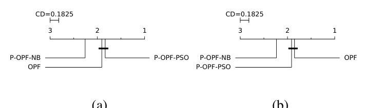
Fig. 3. Comparison between standard OPF and P-OPF with the Nemenyi test concerning the (a) accuracy results and (b) FF-measure values. Groups of techniques that are not significantly different (at p=0.05\mathrm{p}=0.05 ) are connected.
Additionally, we compared the proposed approach using PSO for fine-tuning parameters against probabilistic SVM, the
well-known Bayesian classifier and the Logistic Regression 5{ }^{5}, since PSO was more effective than NB in the previous section. The idea is to perform the very same experimental setup but now considering a SVM classifier with Radial Basis Function (RBF) kernel, the Logistic Regression and Bayesian classifier with isotonic calibration 6{ }^{6}. The parameters for SVM 7{ }^{7} and Logistic Regression 8{ }^{8} are fine-tuned through a cross-validation procedure over a validation set using a gridsearch. In order to fulfill such purpose, we apply the same procedure, i.e., a 40:20:4040: 20: 40 range for training, validating, and testing sets, respectively, repeated 30 times (cross-validation) each. Tables V, VI, and VII present the mean accuracy, FF measure results and Log loss values, respectively. The values in bold stand for the most accurate techniques according to the Wilcoxon signed-rank test.
TABLE V
MEAN ACCURACY RESULTS CONSIDERING BAYES, LOGISTIC, P-OPF-PSO, AND SVM TECHNIQUES.
| Dataset | Bayes | Logistic Regression | P-OPF-PSO | SVM |
|---|---|---|---|---|
| UCI-Adult | 53.38±7.6053.38 \pm 7.60 | 76.13±0.45\mathbf{7 6 . 1 3} \pm 0.45 | 67.42±1.0267.42 \pm 1.02 | 75.80±0.6475.80 \pm 0.64 |
| Statlog-Australian | 84.42±1.3684.42 \pm 1.36 | 86.28±1.13\mathbf{8 6 . 2 8} \pm 1.13 | 78.35±2.0078.35 \pm 2.00 | 85.70±1.4585.70 \pm 1.45 |
| Pima-Indians-Diabetes | 70.43±2.3170.43 \pm 2.31 | 71.95±2.00\mathbf{7 1 . 9 5} \pm 2.00 | 63.36±8.0163.36 \pm 8.01 | 71.39±2.52\mathbf{7 1 . 3 9} \pm 2.52 |
| UCI-Ionosphere | 87.53±3.7387.53 \pm 3.73 | 83.41±3.1883.41 \pm 3.18 | 78.57±12.0478.57 \pm 12.04 | 92.62±4.15\mathbf{9 2 . 6 2} \pm 4.15 |
| UCI-Lenkemia | 93.86±4.16\mathbf{9 3 . 8 6} \pm 4.16 | 86.30±18.29\mathbf{8 6 . 3 0} \pm 18.29 | 75.73±16.1475.73 \pm 16.14 | 84.56±20.96\mathbf{8 4 . 5 6} \pm 20.96 |
| UCI-Liver-disorders | 57.36±3.3457.36 \pm 3.34 | 62.84±6.6462.84 \pm 6.64 | 60.13±4.9060.13 \pm 4.90 | 64.97±4.39\mathbf{6 4 . 9 7} \pm 4.39 |
| UCI-Madelon | 59.44±1.15\mathbf{5 9 . 4 4} \pm 1.15 | 55.73±1.4455.73 \pm 1.44 | 52.72±1.3852.72 \pm 1.38 | 50.50±2.0950.50 \pm 2.09 |
| UCI-Sonar | 72.80±6.1972.80 \pm 6.19 | 75.11±5.0975.11 \pm 5.09 | 82.21±4.33\mathbf{8 2 . 2 1} \pm 4.33 | 77.04±5.7377.04 \pm 5.73 |
| UCI-Splice | 50.15±0.2850.15 \pm 0.28 | 50.00±0.0050.00 \pm 0.00 | 55.99±1.63\mathbf{5 5 . 9 9} \pm 1.63 | 50.67±0.5450.67 \pm 0.54 |
| Synthetic01 | 53.69±2.1653.69 \pm 2.16 | 49.03±2.7049.03 \pm 2.70 | 60.99±1.82\mathbf{6 0 . 9 9} \pm 1.82 | 58.10±4.6358.10 \pm 4.63 |
| Synthetic02 | 64.46±6.5764.46 \pm 6.57 | 49.22±6.4149.22 \pm 6.41 | 90.30±1.54\mathbf{9 0 . 3 0} \pm 1.54 | 90.86±1.72\mathbf{9 0 . 8 6} \pm 1.72 |
As one can observe in Table V, the SVM probabilistic, Logistic classifier, and P-OPF showed close results, in which SVM achieved the best results in 2 datasets (i.e., the “UCIIonosphere” and “UCI-Liver-disorders”) and similar accuracies in 3 out of 11 datasets, while the Logistic Regression achieved the best results in 2 datasets (i.e., the “UCI-Adult” and “Statlog-Australian”), and similar accuracies in 2 out of 11 datasets. Regarding P-OPF, it obtained better results in 3 datasets (i.e., “UCI-Sonar”, “UCI-Splice”, and “Synthetic01”), and similar accuracies in 1 out of 11 datasets. The FF-measure statistical analysis (Table VI) showed a similar results to the ones obtained by standard accuracy, except for "UCI-Liverdisorders " dataset, which was better generalized by SVM and Logistic Regression as well.
We also considered evaluating the techniques using the log loss measure LL, which is formulated as follows:
L=−1m∑i=1m(yilog(pi)+(1−yi)log(1−pi))L=-\frac{1}{m} \sum_{i=1}^{m}\left(y_{i} \log \left(p_{i}\right)+\left(1-y_{i}\right) \log \left(1-p_{i}\right)\right)
Notice the above formula stands for the average value of F(θ)F(\theta) (Equation 4). Table VII presents the results concerning the log loss function. As one can observe, probabilistic SVM showed the best results but being closely followed by P-OPF-NB. The
- 5{ }^{5} We used the SVM probabilistic available in the scikit-learn toolkit [32].
6{ }^{6} We used the probability calibration available in the scikit-learn library [32].
7{ }^{7} The RBF parameters were optimized within the ranges γ∈{0.01,0.1,1}\gamma \in\{0.01,0.1,1\} and C∈{1,10,100}C \in\{1,10,100\}.
8{ }^{8} The Logistic Regression parameters were optimized within the ranges penalty =[L1,L2]=[L 1, L 2], solver =[liblinear=[l i b l i n e a r, saga ]] and C∈C \in {0.01,0.1,1,10,100}\{0.01,0.1,1,10,100\}. ↩︎
TABLE VI
MEAN FF-MEASURE VALUES CONSIDERING BAYES, LOGISTIC, P-OPF-PSO, AND SVM TECHNIQUES.
| Dataset | Bayes | Logistic Regression | P-OPF-PSO | SVM |
|---|---|---|---|---|
| UCI-Adult | 0.4556 ±0.0548\pm 0.0548 | 0.7767±0.0637\mathbf{0 . 7 7 6 7} \pm 0.0637 | 0.6384 ±0.0122\pm 0.0122 | 0.7747±0.00500.7747 \pm 0.0050 |
| Statlog-Australian | 0.8422 ±0.0134\pm 0.0134 | 0.8600±0.0106\mathbf{0 . 8 6 0 0} \pm 0.0106 | 0.7840 ±0.0196\pm 0.0196 | 0.8520±0.01430.8520 \pm 0.0143 |
| Pima-Indians-Diabetes | 0.7111 ±0.0225\pm 0.0225 | 0.7280±0.0207\mathbf{0 . 7 2 8 0} \pm 0.0207 | 0.6311 ±0.0896\pm 0.0896 | 0.7243±0.0265\mathbf{0 . 7 2 4 3} \pm 0.0265 |
| UCI-Intosphere | 0.8863 ±0.0340\pm 0.0340 | 0.8470 ±0.0314\pm 0.0314 | 0.8013 ±0.1317\pm 0.1317 | 0.8280±0.0357\mathbf{0 . 8 2 8 0} \pm 0.0357 |
| UCI-Leukemia | 0.9450±0.0352\mathbf{0 . 9 4 5 0} \pm 0.0352 | 0.8369±0.2225\mathbf{0 . 8 3 6 9} \pm 0.2225 | 0.7021 ±0.1734\pm 0.1734 | 0.8196±0.2564\mathbf{0 . 8 1 9 6} \pm 0.2564 |
| UCI-Liver-diseeders | 0.5484 ±0.0570\pm 0.0570 | 0.6069±0.1101\mathbf{0 . 6 0 6 9} \pm 0.1101 | 0.6010 ±0.0496\pm 0.0496 | 0.6452±0.0535\mathbf{0 . 6 4 5 2} \pm 0.0535 |
| UCI-Madelon | 0.5008±0.0114\mathbf{0 . 5 0 0 8} \pm 0.0114 | 0.5572 ±0.0144\pm 0.0144 | 0.5252 ±0.0138\pm 0.0138 | 0.3704±0.07590.3704 \pm 0.0759 |
| UCI-Sonar | 0.7255 ±0.0042\pm 0.0042 | 0.7495 ±0.0512\pm 0.0512 | 0.8235±0.0437\mathbf{0 . 8 2 3 5} \pm 0.0437 | 0.7694 ±0.0584\pm 0.0584 |
| UCI-Splice | 0.4628 ±0.0966\pm 0.0966 | 0.4589 ±0.0060\pm 0.0060 | 0.5472±0.0134\mathbf{0 . 5 4 7 2} \pm 0.0134 | 0.4746±0.01170.4746 \pm 0.0117 |
| Synthesist | 0.5016 ±0.0454\pm 0.0454 | 0.4235 ±0.0780\pm 0.0780 | 0.6097±0.0183\mathbf{0 . 6 0 9 7} \pm 0.0183 | 0.5751±0.05490.5751 \pm 0.0549 |
| Synthesist2 | 0.6309 ±0.0835\pm 0.0835 | 0.4144 ±0.0991\pm 0.0991 | 0.9020±0.0154\mathbf{0 . 9 0 2 0} \pm 0.0154 | 0.9086±0.0173\mathbf{0 . 9 0 8 6} \pm 0.0173 |
issue concerning P-OPF-PSO for some datasets is related to getting trapped from local optima, i.e., we observed that PSO consistently tried to reach the optimum, but not optimizing both parameters AA and BB simultaneously (Equation 11).
TABLE VII
MEAN LOG LOSS VALUES CONSIDERING BAYES, LOGISTIC, P-OPF-NB, P-OPF-PSO, AND SVM CLASSIFIERS.
| Dataset | Bayes | Logistic | P-OPF-NB | P-OPF-PSO | SVM |
|---|---|---|---|---|---|
| UCI-Adult | 0.504 ±0.041\pm 0.041 | 0.327±0.003\mathbf{0 . 3 2 7} \pm 0.003 | 2.068 ±0.137\pm 0.137 | 8.222 ±0.503\pm 0.503 | 0.334 ±0.007\pm 0.007 |
| Statlog-Australian | 0.467 ±0.117\pm 0.117 | 0.368±0.032\mathbf{0 . 3 6 8} \pm 0.032 | 1.017 ±0.105\pm 0.105 | 6.996 ±1.370\pm 1.370 | 0.367±0.032\mathbf{0 . 3 6 7} \pm 0.032 |
| Pima-Indians-Diabetes | 0.509 ±0.129\pm 0.129 | 0.491±0.023\mathbf{0 . 4 9 1} \pm 0.023 | 1.047 ±0.144\pm 0.144 | 9.729 ±0.697\pm 0.697 | 0.492±0.0265\mathbf{0 . 4 9 2} \pm 0.0265 |
| UCI-Intosphere | 0.463 ±0.215\pm 0.215 | 0.594 ±0.012\pm 0.012 | 0.979 ±0.226\pm 0.226 | 4.058 ±1.311\pm 1.311 | 0.266±0.091\mathbf{0 . 2 6 6} \pm 0.091 |
| UCI-Leukemia | 0.208±0.217\mathbf{0 . 2 0 8} \pm 0.217 | 0.205±0.213\mathbf{0 . 2 0 5} \pm 0.213 | 9.404 ±0.148\pm 0.148 | 7.265 ±5.845\pm 5.845 | 0.273±0.220\mathbf{0 . 2 7 3} \pm 0.220 |
| UCI-Liver-diseeders | 0.731 ±0.176\pm 0.176 | 0.631 ±0.028\pm 0.028 | 1.999 ±0.441\pm 0.441 | 12.49 ±2.322\pm 2.322 | 0.615±0.027\mathbf{0 . 6 1 5} \pm 0.027 |
| UCI-Madelon | 0.665±0.007\mathbf{0 . 6 6 5} \pm 0.007 | 0.815 ±0.128\pm 0.128 | 2.740 ±0.080\pm 0.080 | 16.32 ±0.477\pm 0.477 | 0.692 ±0.002\pm 0.002 |
| UCI-Sonar | 0.627 ±0.197\pm 0.197 | 0.667 ±0.318\pm 0.318 | 0.648 ±0.153\pm 0.153 | 5.989 ±1.450\pm 1.450 | 0.478±0.095\mathbf{0 . 4 7 8} \pm 0.095 |
| UCI-Splice | 0.382±0.020\mathbf{0 . 3 8 2} \pm 0.020 | 0.426 ±0.000\pm 0.000 | 1.383 ±0.145\pm 0.145 | 8.335 ±0.411\pm 0.411 | 0.498 ±0.009\pm 0.009 |
| Synthesist | 0.712 ±0.046\pm 0.046 | 0.694 ±0.001\pm 0.001 | 3.456 ±0.503\pm 0.503 | 4.635 ±2.405\pm 2.405 | 0.660±0.012\mathbf{0 . 6 6 0} \pm 0.012 |
| Synthesist2 | 0.646 ±0.025\pm 0.025 | 0.694 ±0.001\pm 0.001 | 0.623 ±0.236\pm 0.236 | 0.796 ±0.582\pm 0.582 | 0.219±0.026\mathbf{0 . 2 1 9} \pm 0.026 |
In regard to the statistical analysis considering the accuracy results (Figure 4a) and FF-measure values (Figure 4b), probabilistic SVM can be considered the most accurate one by Nemenyi test. Furthermore, the statistical test did not point out a CD between the Logistic Regression, P-OPF-PSO, and Bayes, which means they performed similarly.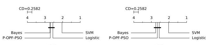
(a)
(b)
Fig. 4. Comparison concerning P-OPF-PSO against Bayes, Logistic Regression, and SVM concerning the Nemenyi test for: (a) accuracy results and (b) FF-measure values.
Table VIII presents the mean computational load (in seconds) for the training and validating phases concerning Bayes, Logistic, P-OPF-PSO, and probabilistic SVM. It is worth noting that the P-OPF and probabilistic SVM have an additional time for training the model due to the calibration of probabilistic predictions according to the Platt scaling. For that purpose, the calibration is performed over a validation set.
Figure 5 shows the statistical analysis considering the computational load for the training time (training and validating) with Nemenyi test. As one can observe, both P-OPF-PSO and SVM are the slowest approaches, since SVM uses the gridsearch to fine-tune the hyper-parameters C,γC, \gamma, followed by the Platt scaling procedure, and P-OPF-PSO is a swarm-based technique, which means an extra computational load to finetune parameters AA and BB. On the average, the fastest approach
TABLE VIII
COMPUTATIONAL LOAD (IN SECONDS) CONCERNING BAYES, LOGISTIC, P-OPF-PSO, AND SVM WITH RESPECT TO THE TRAINING TIME (TRAINING AND VALIDATING).
| Dataset | Bayes | Logistic | P-OPF-PSO | SVM |
|---|---|---|---|---|
| UCI-Adult | 0.1783 ±0.0701\pm 0.0701 | 72.69 ±22.85\pm 22.85 | 242.50 ±36.63\pm 36.63 | 3129.63 ±3603.51\pm 3603.51 |
| Statlog-Australian | 0.0108 ±0.0005\pm 0.0005 | 0.3121 ±0.0498\pm 0.0498 | 0.6331 ±0.0075\pm 0.0075 | 0.3555 ±0.1237\pm 0.1237 |
| Pima-Indians-Diabetes | 0.0111 ±0.0008\pm 0.0008 | 0.2457 ±0.0157\pm 0.0157 | 0.6950 ±0.0066\pm 0.0066 | 0.6645 ±0.3984\pm 0.3984 |
| UCI-Intosphere | 0.0105 ±0.0006\pm 0.0006 | 0.3110 ±0.0169\pm 0.0169 | 0.3169 ±0.0033\pm 0.0033 | 0.1699 ±0.0086\pm 0.0086 |
| UCI-Leukemia | 0.0270 ±0.0033\pm 0.0033 | 4.3729 ±0.5890\pm 0.5890 | 0.1175 ±0.0044\pm 0.0044 | 0.3915 ±0.0228\pm 0.0228 |
| UCI-Liver-diseeders | 0.0101 ±0.0004\pm 0.0004 | 0.2261 ±0.0070\pm 0.0070 | 0.3148 ±0.0100\pm 0.0100 | 0.2615 ±0.1239\pm 0.1239 |
| UCI-Madelon | 0.0425 ±0.0012\pm 0.0012 | 10.46 ±1.2897\pm 1.2897 | 6.1343 ±0.0343\pm 0.0343 | 48.65 ±67.14\pm 67.14 |
| UCI-Sonar | 0.0104 ±0.0005\pm 0.0005 | 0.2970 ±0.0140\pm 0.0140 | 0.1947 ±0.0035\pm 0.0035 | 0.1513 ±0.0048\pm 0.0048 |
| UCI-Splice | 0.0178 ±0.0011\pm 0.0011 | 1.5474 ±0.3463\pm 0.3463 | 3.9445 ±0.0251\pm 0.0251 | 27.56 ±10.89\pm 10.89 |
| Synthesist2 | 0.0108 ±0.0007\pm 0.0007 | 0.2158 ±0.0067\pm 0.0067 | 0.9663 ±0.0802\pm 0.0802 | 0.4485 ±0.0766\pm 0.0766 |
| Synthesist2 | 0.0108 ±0.0005\pm 0.0005 | 0.2139 ±0.0055\pm 0.0055 | 0.9415 ±0.0074\pm 0.0074 | 0.3187 ±0.0143\pm 0.0143 |
(Bayesian classifier) required 0.0309±0.04750.0309 \pm 0.0475 seconds for training, while probabilistic SVM needed 291.69±897.56291.69 \pm 897.56 seconds. P-OPF-PSO performed the training and validating phase in 23.43±69.6123.43 \pm 69.61 seconds, which means it is quite less costly than SVM, mainly due to large datasets employed for comparison purposes (i.e., “UCI-Adult”, “UCI-Madelon”, and “UCI-Splice”). Note that the P-OPF computational load can be optimized using other meta-heuristic-driven techniques.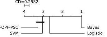
Fig. 5. Comparison concerning P-OPF-PSO, Bayes, Logistic Regression, and SVM with the Nemenyi test considering the computational load for training (training and validating).
B. Experiments for NTL Detection
In this section, we present the experiments results concerning the task of automatic NTL detection. We employed two private datasets from a Brazilian electric utility, being one with 3,182 profiles of industrial consumers ( 2,985 legal and 197 illegal profiles) and the other with 4,952 profiles of commercial consumers ( 4,682 legal and 270 illegal profiles), both represented by eight features:
Demand Billed (DB): demand value of the active power considered for billing purposes, in kilowatts ( kW );
Demand Contracted (DC): the value of the demand for continuous availability requested from the electric utility, in kilowatts ( kW );
Demand Measured or Maximum Demand ( Dmax \mathrm{D}_{\text {max }} ): the maximum actual demand for active power, verified by measurement at fifteen-minute intervals during the billing period, in kilowatts ( kW );
Reactive Energy (RE): energy that flows through the electric and magnetic fields of an AC system, in kilovoltamperes reactive hours ( kVArh );
Power Transformer (PT): the power transformer installed for the consumers, in kilovolt-amperes (kVA);
Power Factor (PF): the ratio between the consumed active and apparent power in a circuit. The PF indicates the efficiency of a power distribution system;
Installed Power ( Pinst \mathrm{P}_{\text {inst }} ): the sum of the nominal power of all electrical equipment installed and ready to operate at the consumer unit, in kilowatts ( kW );
Load Factor (LF): the ratio between the average demand ( Daverage D_{\text {average }} ) and maximum demand ( DmaxD_{\max } ) of the consumer unit. The LFL F is an index that shows how the electric energy is used in a rational way.
At every 15 minutes, the electric utility recorded consumption data during one year. After that, such technical data was used to compute the aforementioned monthly features for both datasets.
Figure 6 depicts the pipeline adopted in this work to validate the proposed probabilistic OPF in the context of automatic non-technical losses identification. Given the profiles collected by the energy company accordingly to their category (i.e., industrial or residential), we can perform the feature extraction step that aims at compiling the above eight features from each consumer. Further, these features will be used as input to P-OPF to learn the correct mapping between a particular profile and its situation in the system, i.e., “legal” or 'llegal" consumer. The outcome of the pipeline is a probability of that profile being a fraudster.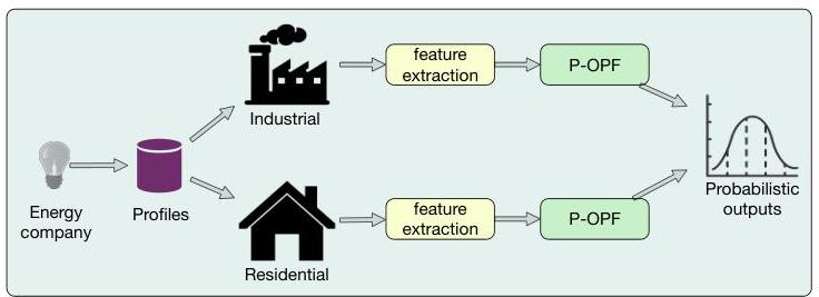
Fig. 6. Pipeline used to validate the proposed approach in the context of NTL identification.
Tables IX and X present the results concerning the task of NTL detection with respect to the accuracy and F-measure values, respectively. Clearly, one can observe that standard OPF and P-OPF-PSO obtained the best results considering the accuracy and F-measure values, and outperformed the other classifiers considerably. However, with respect to the Log loss values, the SVM probabilistic has been a more confidence technique, as one can observe in Table XI.
TABLE IX
MEAN ACCURACY RESULTS OF BAYES, LOGISTIC, P-OPF, OPF AND PROBABILISTIC SVM CONCERNING THE TASK OF NTL DETECTION.
| Dataset | Bayes | Logistic | P-OPF-NB | P-OPF-PSO | OPF | SVM |
|---|---|---|---|---|---|---|
| Commercial | 52.28±1.2652.28 \pm 1.26 | 50.20±0.4750.20 \pm 0.47 | 77.45±3.4877.45 \pm 3.48 | 83.41±2.34\mathbf{8 3 . 4 1} \pm 2.34 | 83.41±2.34\mathbf{8 3 . 4 1} \pm 2.34 | 56.02±7.3556.02 \pm 7.35 |
| Industrial | 52.38±1.3052.38 \pm 1.30 | 50.36±0.8050.36 \pm 0.80 | 73.68±3.5773.68 \pm 3.57 | 80.78±2.7180.78 \pm 2.71 | 80.80±2.71\mathbf{8 0 . 8 0} \pm 2.71 | 58.22±7.2158.22 \pm 7.21 |
TABLE X
MEAN F-MEASURE VALUES OF BAYES, LOGISTIC, P-OPF, OPF AND PROBABILISTIC SVM CONCERNING THE TASK OF NTL DETECTION.
| Dataset | Bayes | Logistic | P-OPF-NB | P-OPF-PSO | OPF | SVM |
|---|---|---|---|---|---|---|
| Commercial | 0.530±0.0230.530 \pm 0.023 | 0.493±0.0870.493 \pm 0.087 | 0.788±0.0280.788 \pm 0.028 | 0.820±0.018\mathbf{0 . 8 2 0} \pm 0.018 | 0.820±0.018\mathbf{0 . 8 2 0} \pm 0.018 | 0.577±0.0860.577 \pm 0.086 |
| Industrial | 0.528±0.0230.528 \pm 0.023 | 0.489±0.0170.489 \pm 0.017 | 0.758±0.0260.758 \pm 0.026 | 0.800±0.019\mathbf{0 . 8 0 0} \pm 0.019 | 0.801±0.019\mathbf{0 . 8 0 1} \pm 0.019 | 0.625±0.1010.625 \pm 0.101 |
From such results, one can draw som interesting conclusions: firstly, probabilistic OPF can provide results that are
TABLE XI
MEAN LOG LOSS VALUES OF BAYES, LOGISTIC, P-OPF AND PROBABILISTIC SVM CONCERNING THE TASK OF NTL DETECTION.
| Dataset | Bayes | Logistic | P-OPF-NB | P-OPF-PSO | SVM |
|---|---|---|---|---|---|
| Commercial | 0.206±0.0130.206 \pm 0.013 | 0.214±0.0100.214 \pm 0.010 | 0.426±0.0620.426 \pm 0.062 | 0.829±0.2860.829 \pm 0.286 | 0.183±0.033\mathbf{0 . 1 8 3} \pm 0.033 |
| Industrial | 0.222±0.0250.222 \pm 0.025 | 0.237±0.0180.237 \pm 0.018 | 0.422±0.0850.422 \pm 0.085 | 0.976±0.3400.976 \pm 0.340 | 0.187±0.036\mathbf{0 . 1 8 7} \pm 0.036 |
similar to is standard version, but with the benefit of soft (i.e., probabilistic) outputs. Such skill plays an important role in the context of NTL identification, where the probability of being an illegal consumer is sometimes more interesting than just labeling it as a thief or not. Secondly, probabilistic OPF outperformed SVM by far if we consider the accuracy and FF-measure, thus showing to be robust enough to be compared to state-of-the-art techniques.
V. CONCLUSIONS AND FUTURE WORKS
Probabilistic classification has been a topic of great interest concerning the machine learning community, mainly due to the lack of a more “flexible” information rather than labels only. In this work, we cope with this problem by proposing a probabilistic OPF for NTL detection, namely P-OPF. The results of the proposed P-OPF were compared against standard OPF, probabilistic SVM, the well-known Bayesian classifier, and the Logistic Regression in a number of datasets, achieving suitable results in several of them.
In regard to future works, we aim at extending P-OPF for multi-class classification problems, as well as to consider other optimization techniques to fine-tune the new parameters that help minimizing the cost function.
ACKNOWLEDGMENTS
The authors would like to thank Capes, CNPq grants #306166/2014-3 and #307066/2017-7, as well as FAPESP grants #2013/07375-0, #2014/16250-9, #2014/12236-1, #2016/19403-6, and #2017/02286-0.
ACRONYMS
| SVM | Support Vector Machines |
|---|---|
| NTL | Non-Technical Losses |
| OPF | Optimum-Path Forest |
| OPT | Optimum-Path Tree |
| P-OPF | Probabilistic Optimum-Path Forest |
| PSO | Particle Swarm Optimization |
| NB | Newton Backtracking optimizer |
| P-OPF-PSO | P-OPF optimized with PSO |
| P-OPF-NB | P-OPF optimized with NB |
REFERENCES
[1] J. C. Platt, “Probabilistic outputs for support vector machines and comparisons to regularized likelihood methods,” in Advances in Large Margin Classifiers. MIT Press, 1999, pp. 61-74.
[2] C. C. O. Ramos, A. N. Souza, A. X. Falcão, and J. P.Papa, “New insights on nontechnical losses characterization through evolutionarybased feature selection,” IEEE Transactions on Power Delivery, vol. 27, no. 1, pp. 140-146, 2012.
[3] D. R. Pereira, M. A. Pazoti, L. A. M. Pereira, D. Rodrigues, C. C. O. Ramos, A. N. de Souza, and J. P. Papa, “Social-spider optimizationbased support vector machines applied for energy theft detection,” Computers & Electrical Engineering, vol. 49, pp. 25-38, 2016.
[4] C. C. O. Ramos, D. Rodrigues, A. N. de Souza, and J. P. Papa, “On the study of commercial losses in brazil: A binary black hole algorithm for theft characterization,” IEEE Transactions on Smart Grid, vol. PP, no. 99, pp. 1-1, 2016.
[5] J. B. Leite and J. R. S. Mantovani, “Detecting and locating non-technical losses in modern distribution networks,” IEEE Transactions on Smart Grid, vol. PP, no. 99, pp. 1-1, 2017.
[6] J. L. Viegas, P. R. Esteves, R. Melício, V. M. F. Mendes, and S. M. Vieira, “Solutions for detection of non-technical losses in the electricity grid: A review,” Renewable and Sustainable Energy Reviews, vol. 80, pp. 1256-1268, 2017.
[7] W. Han and Y. Xiao, “A novel detector to detect colluded non-technical loss frauds in smart grid,” Computer Networks, vol. 117, pp. 19-31, 2017, cyber-physical systems and context-aware sensing and computing.
[8] C. H. Lin, S. J. Chen, C. L. Kuo, and J. L. Chen, “Non-cooperative game model applied to an advanced metering infrastructure for non-technical loss screening in micro-distribution systems,” IEEE Transactions on Smart Grid, vol. 5, no. 5, pp. 2468-2469, 2014.
[9] S. Chatterjee, V. Archana, K. Suresh, R. Saha, R. Gupta, and F. Doshi, “Detection of non-technical losses using advanced metering infrastructure and deep recurrent neural networks,” in IEEE International Conference on Environment and Electrical Engineering and 2017 IEEE Industrial and Commercial Power Systems Europe, 2017, pp. 1-6.
[10] T. Ahmad, “Non-technical loss analysis and prevention using smart meters,” Renewable and Sustainable Energy Reviews, vol. 72, pp. 573589, 2017.
[11] J. P. Papa, A. X. Falcão, and C. T. N. Suzuki, “Supervised pattern classification based on optimum-path forest,” International Journal of Imaging Systems and Technology, vol. 19, no. 2, pp. 120-131, 2009.
[12] J. P. Papa, A. X. Falcão, V. H. C. Albuquerque, and J. M. R. S. Tavares, “Efficient supervised optimum-path forest classification for large datasets,” Pattern Recognition, vol. 45, no. 1, pp. 512-520, 2012.
[13] J. P. Papa, S. E. N. Fernandes, and A. X. Falcão, “Optimum-path forest based on k-connectivity: Theory and applications,” Pattern Recognition Letters, 2016.
[14] C. C. O. Ramos, A. N. de Sousa, J. P. Papa, and A. X. F. ao, “A new approach for nontechnical losses detection based on optimum-path forest,” IEEE Transactions on Power Systems, vol. 26, no. 1, pp. 181189, 2011.
[15] L. A. P. Júnior, C. C. O. Ramos, D. Rodrigues, D. R. Pereira, A. N. Souza, K. A. P. Costa, and J. P. Papa, “Unsupervised non-technical losses identification through optimum-path forest,” Electric Power Systems Research, vol. 140, pp. 413-423, 2016.
[16] L. M. Rocha, F. A. M. Cappabianco, and A. X. Falcão, “Data clustering as an optimum-path forest problem with applications in image analysis,” International Journal of Imaging Systems and Technology, vol. 19, no. 2, pp. 50-68, 2009.
[17] R. D. Trevizan, A. S. Bretas, and A. Rossoni, “Nontechnical losses detection: A discrete cosine transform and optimum-path forest based approach,” in 2015 North American Power Symposium (NAPS), 2015, pp. 1-6.
[18] J. I. Guerrero, I. Monedero, F. Biscarri, J. Biscarri, R. Milln, and C. Len, “Non-technical losses reduction by improving the inspections accuracy in a power utility,” IEEE Transactions on Power Systems, vol. PP, no. 99, pp. 1-1, 2017.
[19] S. E. N. Fernandes, W. Scheirer, D. D. Cox, and J. P. Papa, Progress in Pattern Recognition, Image Analysis, Computer Vision, and Applications: 20th Iberoamerican Congress, ser. CIARP '15. Springer International Publishing, 2015, ch. Improving Optimum-Path Forest Classification Using Confidence Measures, pp. 619-625.
[20] S. E. N. Fernandes and J. P. Papa, “Improving optimum-path forest learning using bag-of-classifiers and confidence measures,” Pattern Analysis and Applications, 2017.
[21] W. P. Amorim, A. X. Falcão, J. P. Papa, and M. H. Carvalho, “Improving semi-supervised learning through optimum connectivity,” Pattern Recognition, 2016, (to appear).
[22] J. P. Papa and A. X. Falcão, “A new variant of the optimum-path forest classifier,” in Advances in Visual Computing, ser. Lecture Notes in Computer Science, G. Bebis, R. Boyle, B. Parvin, D. Koracin, P. Remagnino, F. Porikli, J. Peters, J. Klosowski, L. Arns, Y. Chun, T.-M. Rhyne, and L. Monroe, Eds. Springer Berlin Heidelberg, 2008, vol. 5358, pp. 935-944.
[23] ——, “A learning algorithm for the optimum-path forest classifier,” in Graph-Based Representations in Pattern Recognition, ser. Lecture Notes in Computer Science, A. Torsello, F. Escolano, and L. Brun, Eds. Springer Berlin Heidelberg, 2009, vol. 5534, pp. 195-204.
[24] C. Allène, J.-Y. Audibert, M. Couprie, and R. Keriven, “Some links between extremum spanning forests, watersheds and min-cuts,” Image and Vision Computing, vol. 28, no. 10, pp. 1460-1471, 2010, image Analysis and Mathematical Morphology.
[25] A. X. Falcão, J. Stolfi, and R. A. Lotufo, “The image foresting transform: theory, algorithms, and applications,” IEEE Transactions on Pattern Analysis and Machine Intelligence, vol. 26, no. 1, pp. 19-29, 2004.
[26] H.-T. Lin, C.-J. Lin, and R. C. Weng, “A note on platf’s probabilistic outputs for support vector machines,” Machine Learning, vol. 68, no. 3, pp. 267-276, 2007.
[27] D. Goldberg, “What every computer scientist should know about floating-point arithmetic,” ACM Computing Surveys, vol. 23, no. 1, pp. 5−48,19915-48,1991.
[28] J. Kennedy and R. C. Eberhart, Swarm Intelligence. San Francisco, USA: Morgan Kaufmann Publishers Inc., 2001.
[29] F. Wilcoxon, “Individual comparisons by ranking methods,” Biometrics Bulletin, vol. 1, no. 6, pp. 80-83, 1945.
[30] P. Nemenyi, Distribution-free Multiple Comparisons. Princeton University, 1963.
[31] J. Demšar, “Statistical comparisons of classifiers over multiple data sets,” The Journal of Machine Learning Research, vol. 7, pp. 1-30, 2006.
[32] F. Pedregosa, G. Varoquaux, A. Gramfort, V. Michel, B. Thirion, O. Grisel, M. Blondel, P. Prettenhofer, R. Weiss, V. Dubourg, J. Vanderplas, A. Passos, D. Cournapeau, M. Brucher, M. Perrot, and E. Duchesnay, “Scikit-learn: Machine learning in Python,” Journal of Machine Learning Research, vol. 12, pp. 2825-2830, 2011.