Service District Optimization: Usage of Facility Location Methods and Geographic Information Systems to Analyze and Optimize Urban Food Retail Distribution (original) (raw)
Abstract
With the surge of obesity in the United States, improving urban food environments has gained in importance. Research on food deserts focuses mainly on assessing the food environment but lacks methods of generating good solutions for the placement of food stores. This work uses a maximum covering location problem in combination with census block group GIS data from the City of Philadelphia to find optimal locations for future food store openings. A socioeconomic index of vulnerability is computed to weigh regions based on their residents' sensitivity to food access limitations. The analysis found that supermarkets in Philadelphia are relatively unequally distributed and that there are many viable locations which could satisfy both the public interest of improving food access as well as the private interest of being profitable. Going forward, this joint approach of GIS data and operations research can be used to highlight locations for possible policy interventions in urban areas.
Figures (26)
tion A multi-level study surveyed 15,358 inhabitants of 327 zip code tabulation areas in Mas- sachusetts, USA between 1998 and 2002 (Lopez| 2007). The presence of a supermarket was negatively associated with obesity risk. In a mul supermarket in a zip code tabulation area decreased t +1000 per square mile), and retail es- As median income (+$1000), population density tablishment density (+100 per square mile) increased, t 2%, and 1.9%. tiple regression model, having one he risk of obesity by 10.7 percent. he risk of obesity declined by 0.8%,
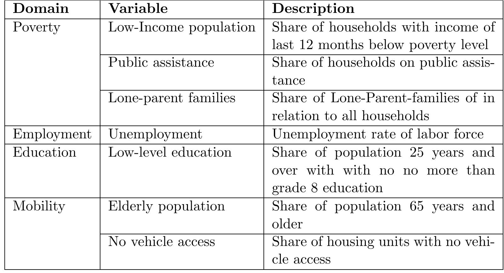
Table 3.1.: Socioeconomic variables of neighborhood vulnerability Table 3.2.: Descriptive statistics of vulnerability variables in block groups of Philadelphia
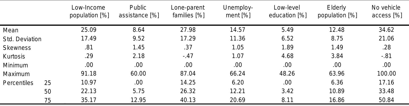
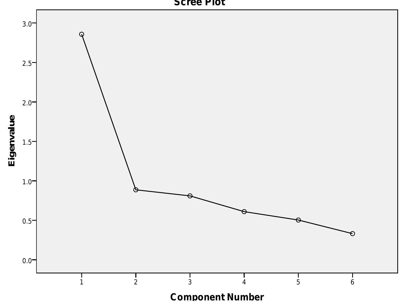
Figure 3.1.: Scree plot from eigenvalues of factors The resulting component loadings using are shown in the component matrix in/3.4| Because only one component is retained, the solution has not been rotated. The factor loadings
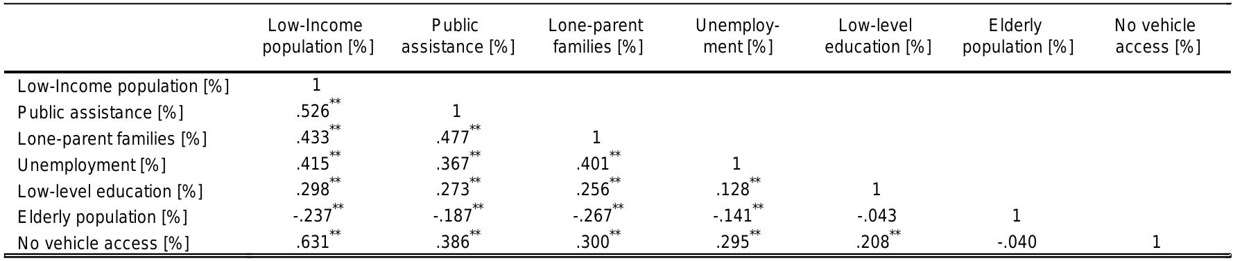
Table 3.3.: Pearson correlations of vulnerability variables in block groups of Philadelphia **. Correlation is significant at the 0.01 level (2-tailed).
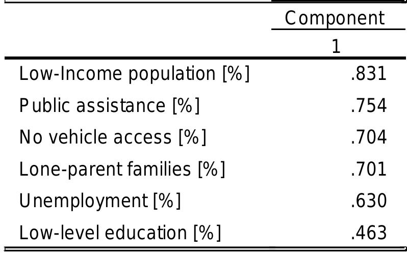
Table 3.4.: Principal Factor Analysis component matrix Extraction Method: Principal Component Analvsis represent both the weighting of variables for each factor but also the correlation between the variables and the factor.
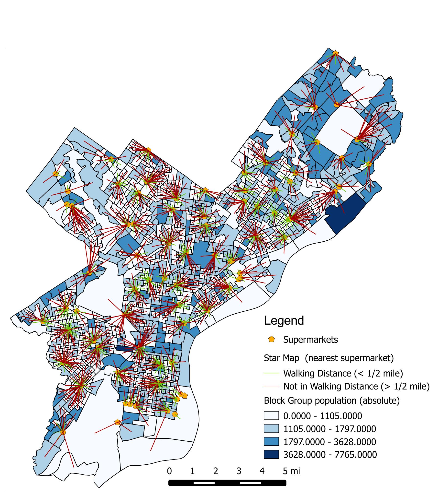
Figure 4.2.: Star Map of nearest supermarket per Block Group centroid
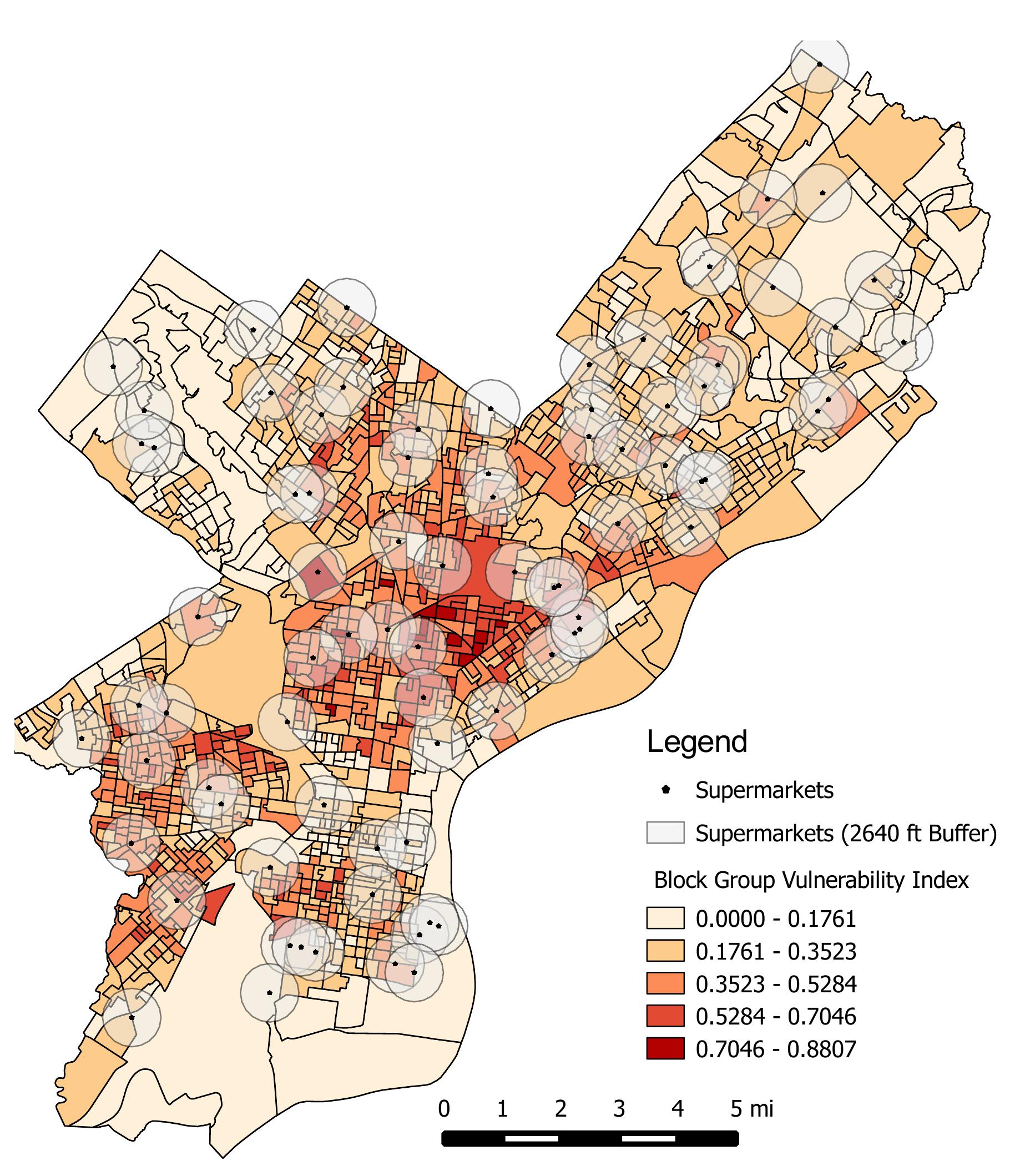
Figure 4.3.: Map of Block Group level Vulnerability and supermarket coverage areas
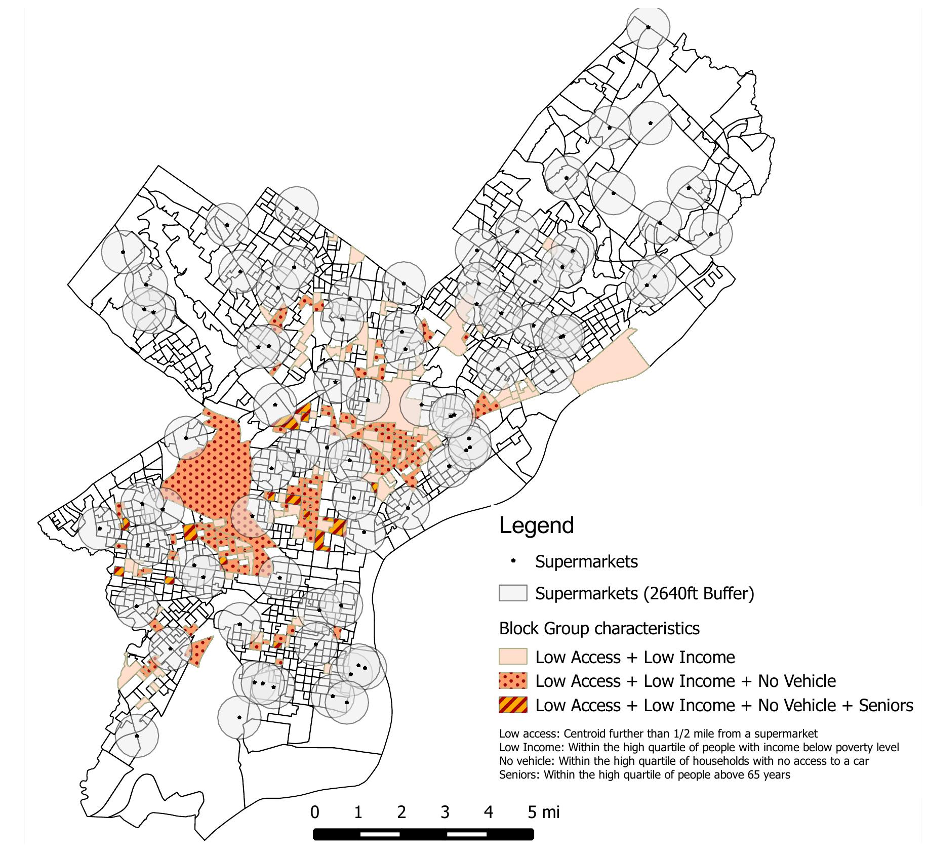
Figure 4.4.: Map of Combinations of Vulnerability characteristics
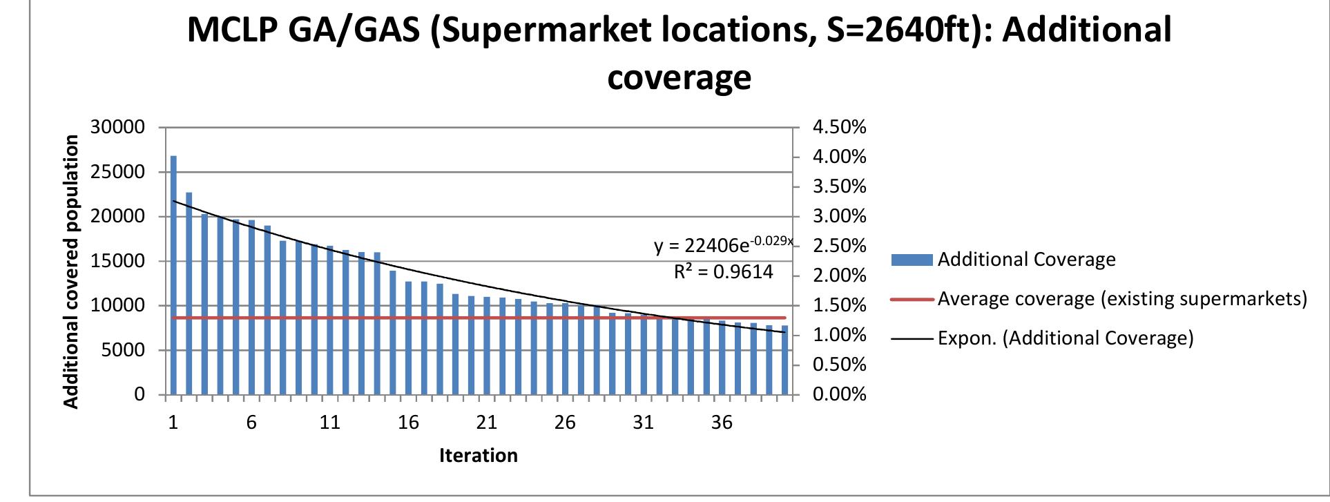
Figure 4.5.: 40-MCLP of supermarket placement coverage graph
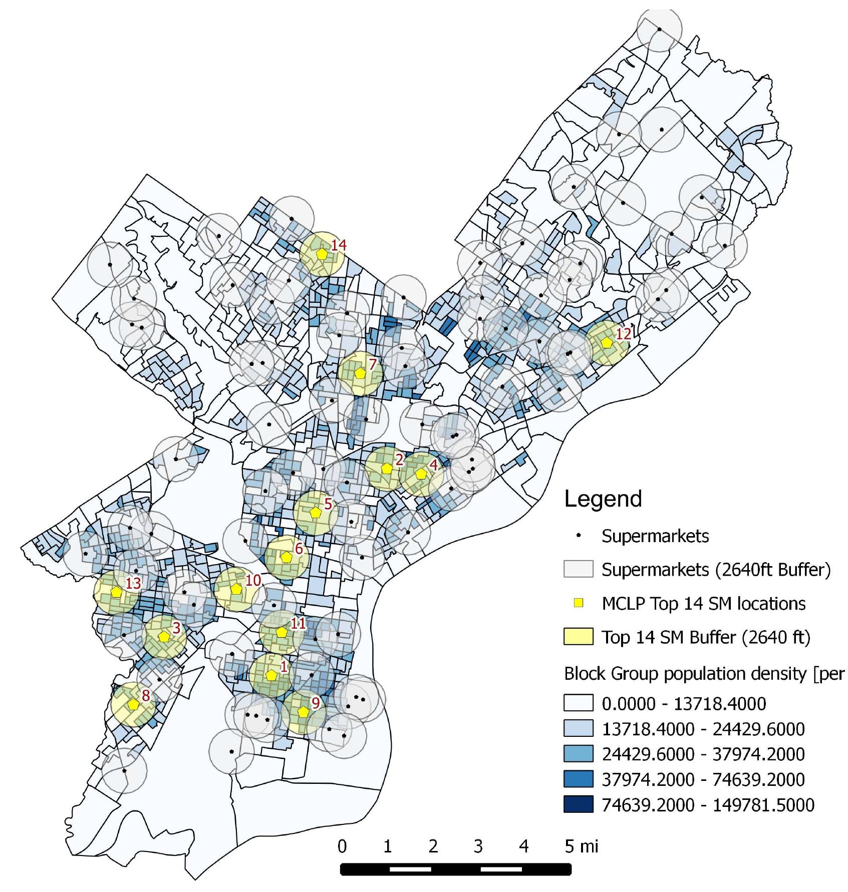
Figure 4.6.: Map of optimal 14 MCLP locations (placement: Supermarkets, p=40, initial coverage: supermarkets (S=4 mile)
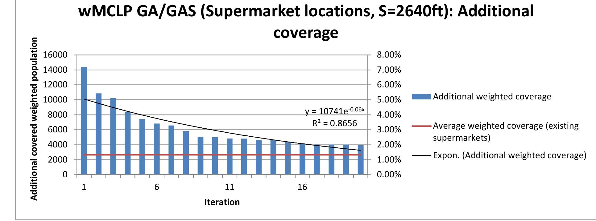
Figure 4.7.: 20-wMCLP of supermarket placement coverage graph
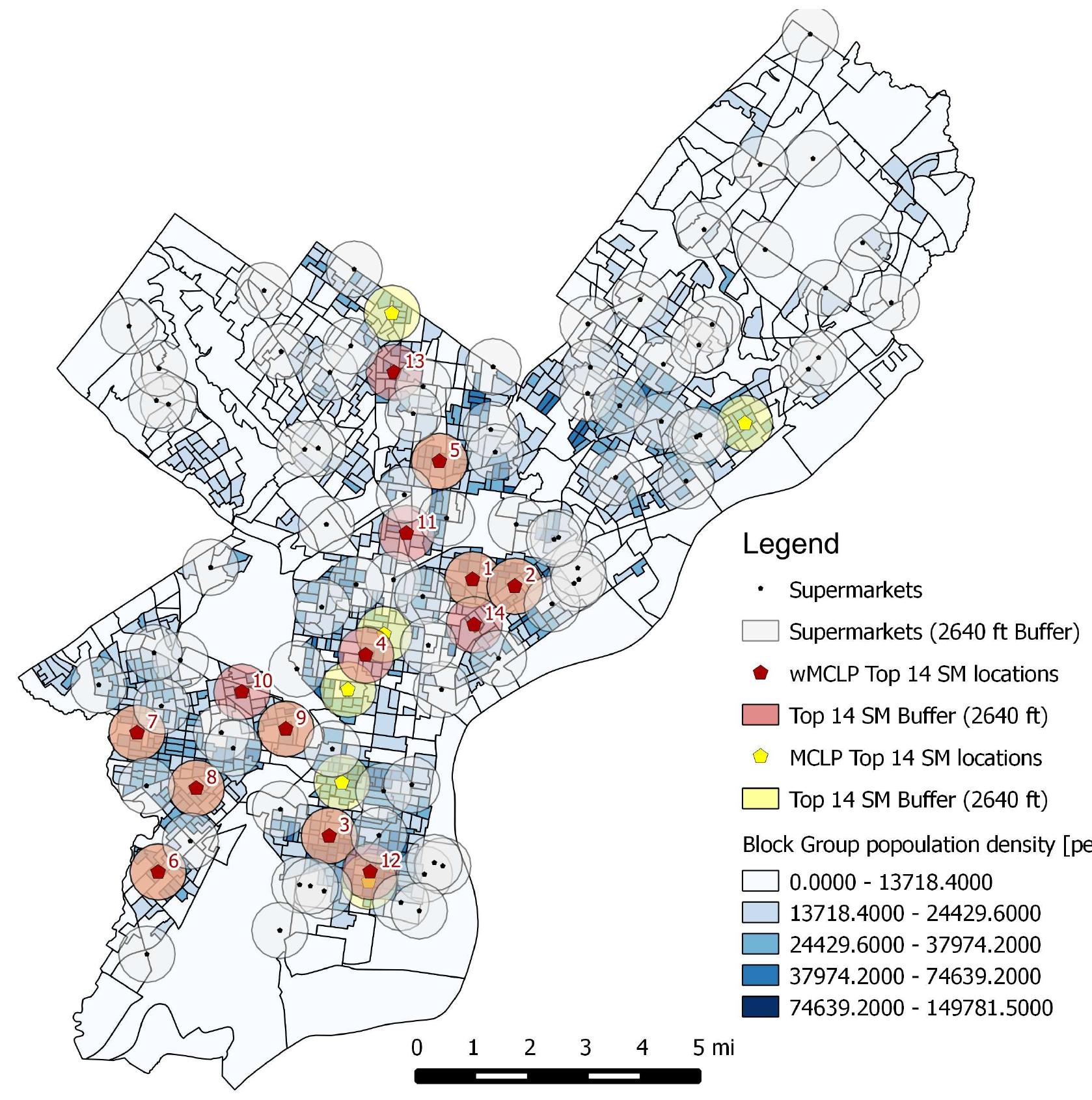
Figure 4.8.: Map of optimal 14 wMCLP locations in comparison to MCLP locations (place- ment: Supermarkets, p=40, initial coverage: supermarkets (S=3 mile)
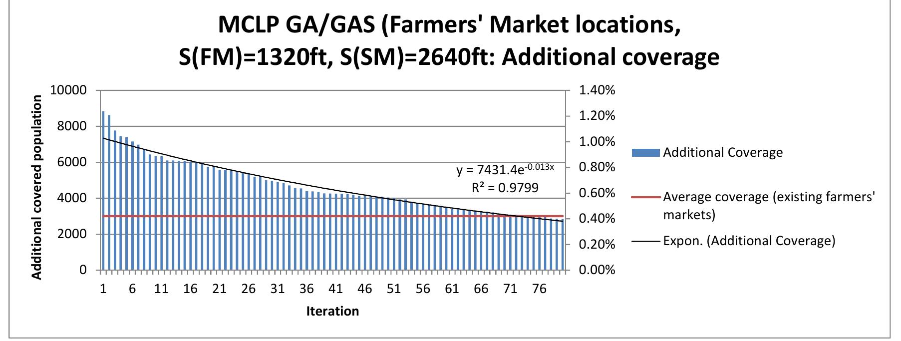
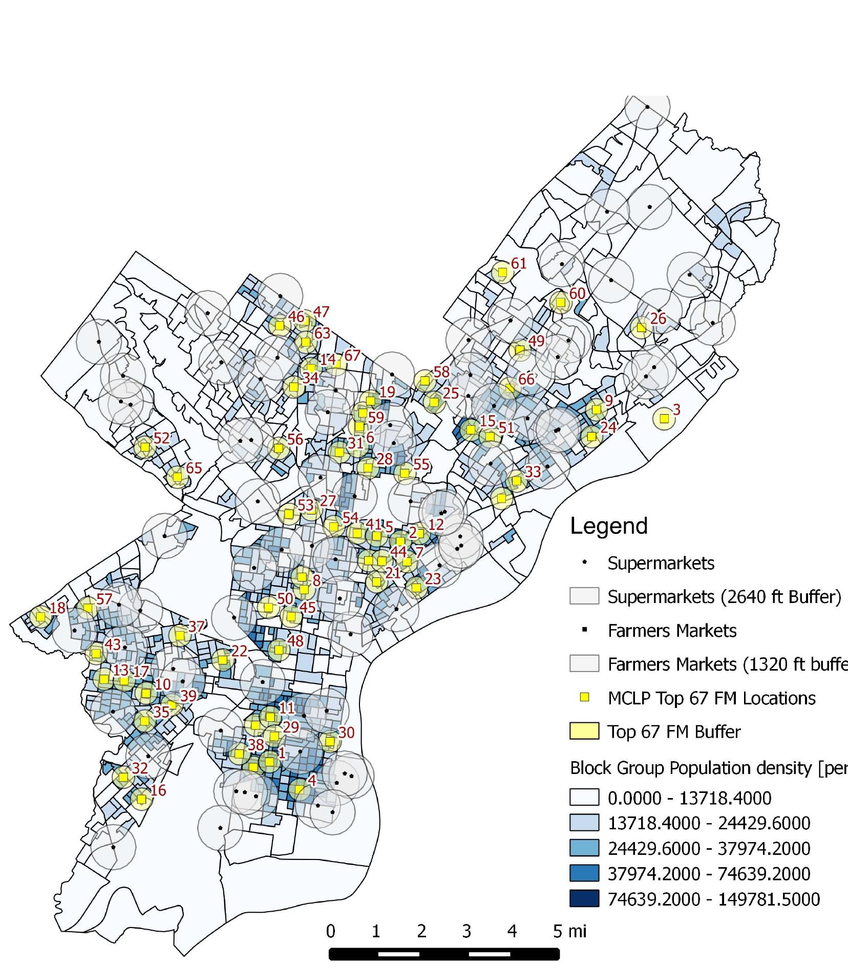
resulting list of facilities is ranked by contribution to the objective function and that the objective value of the GA heuristic solution is identical to value of the GAS heuristic solution. The coverage graph in Figure /4.9 reveals that openings of 67 Farmers’ Markets would yield above-average coverage. That is surprising, considering that the coverage ot existing Farmers’ Markets was calculated based on a no competition from supermarkets. while the new located Farmers’ Markets’ coverage only consists of areas that are left uncovered by existing Farmers’ Markets as well as supermarkets. Reasons for this anomaly could include the inefficient placement of existing Farmers’ Markets, a too small buffer in correspondence to too large subdivisions (Block Groups) or the aggregation of several Farmers’ Markets in the city center, leading to overlapping areas of coverage. A map ot the above-mentioned 67 Farmers’ Markets is another sign for the amount of demand fot food that is not satisfied in high-density areas, as new facility proposals concentrate on areas with high relative density (see Figure 4.10). Figure 4.9.: 80-MCLP of farmers’ market placement coverage graph
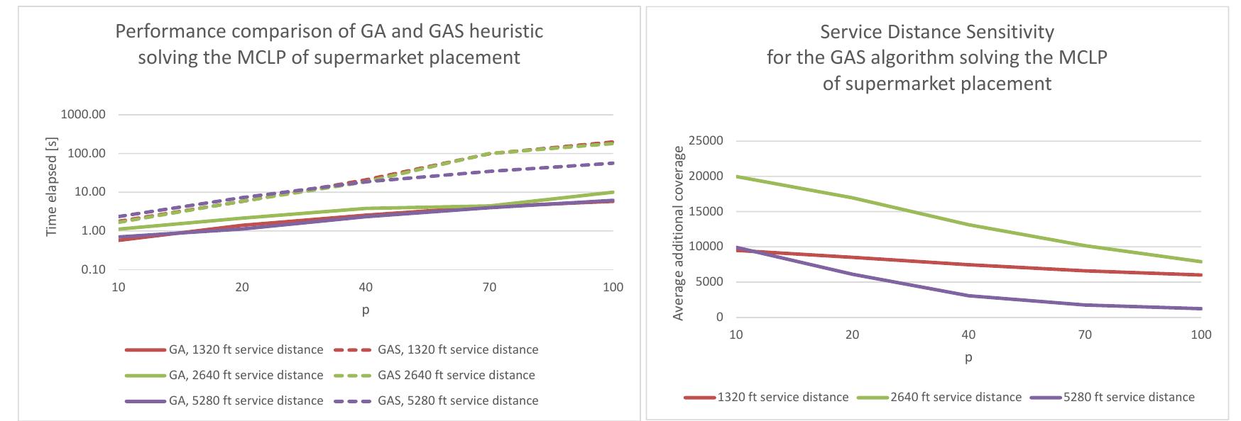
algorithm would find. Both algorithms were written parametric, such that they allowed for quick change of input parameters. The trade-off is a higher computation time for the Substitution heuristic, as the amount of pairwise combinations of locations to be checked increases with the iterations (set by the value of p). The values of p (possible facility open- ings) that were relevant for this application were fairly small, because certain feasibility constraints for new store openings were applied (such as above-average new coverage). The algorithms were run in MATLAB R2013b on a 2.0 GHz Intel Core 2 Duo laptop with 3GB of memory running Windows 7 (64 Bit) with service pack 1. Tables |4.1| and |4.2 depict several runs of both algorithms. In the MCLP, the first swap of locations was only done in the 46‘ iteration. Hence, only for values higher than 46 would the GAS yield an improvement but overall takes much longer computing time (e.g. increasing the value of p by the factor five from 20 to 100 lead to a computing time increase by the factor of five for the GA heuristic and a computing time increase by the factor of 31 for the GAS heuristic. For the performance test of the SCLP algorithm, the buffer sizes were varied. This had two effects: First, the amount of necessary facilities increases because of the smaller coverage area and second, the amount nodes to be covered increases as well. Higher values of p result in more opportunities for Substitutions, so the GAS solutions need a smaller amount of facilities to cover the whole demand point set (2.2 percent and 4.7 percent respectively). However, the general computing time of the GAS algorithm is higher and furthermore increases more strongly with decreasing buffer size. A maximal service distance of 5; tech- nically inducing the problem of trying to cover all demand points by placing supermarkets, takes a computing time of over five minutes. Cutting the service distance in half took more than ten times the computing time. In theory, the GAS algorithm yields better objective function values in exchange for more computing time. For this application, the improvement through substitution did not mat- ter for the values of p that were constrained by the minimum coverage constraints. Hence, the GAS heuristic could only be used as an affirmation of the good solution provided by el... £4... UI. COCOA UT... EDCUrg 1... 2 Le
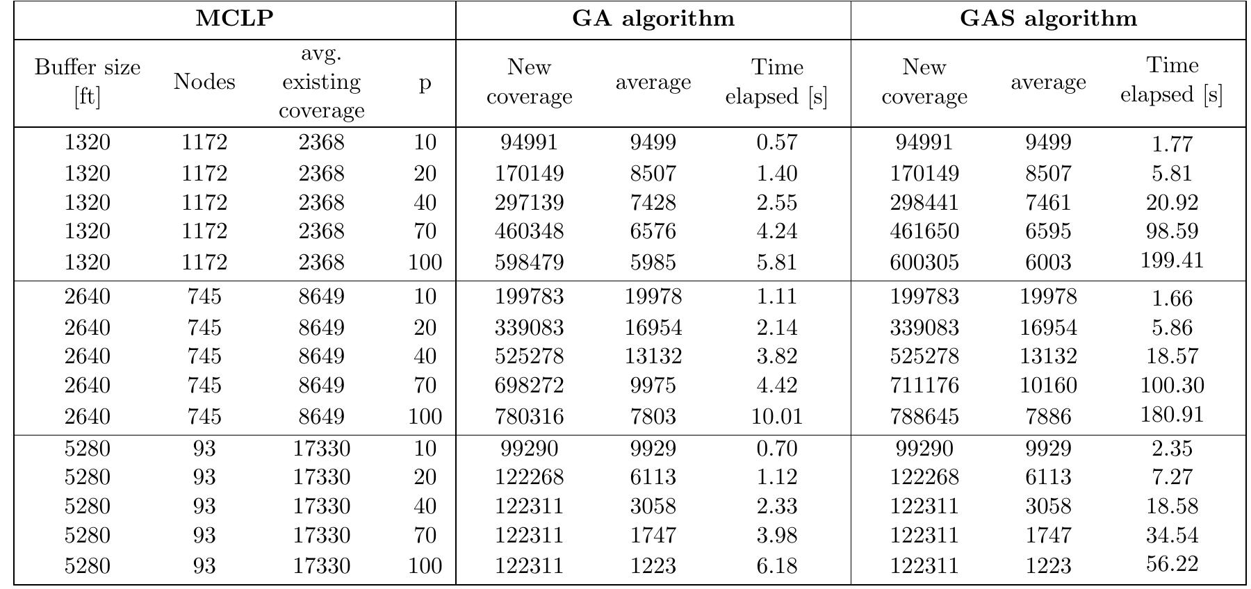
Table 4.1.: Performance and Sensitivities of algorithms for a MCLPs Table 4.2.: Performance and Sensitivities of algorithms for SCLPs
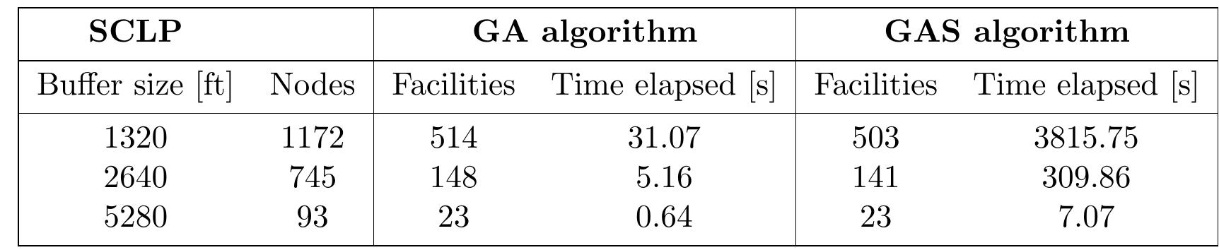
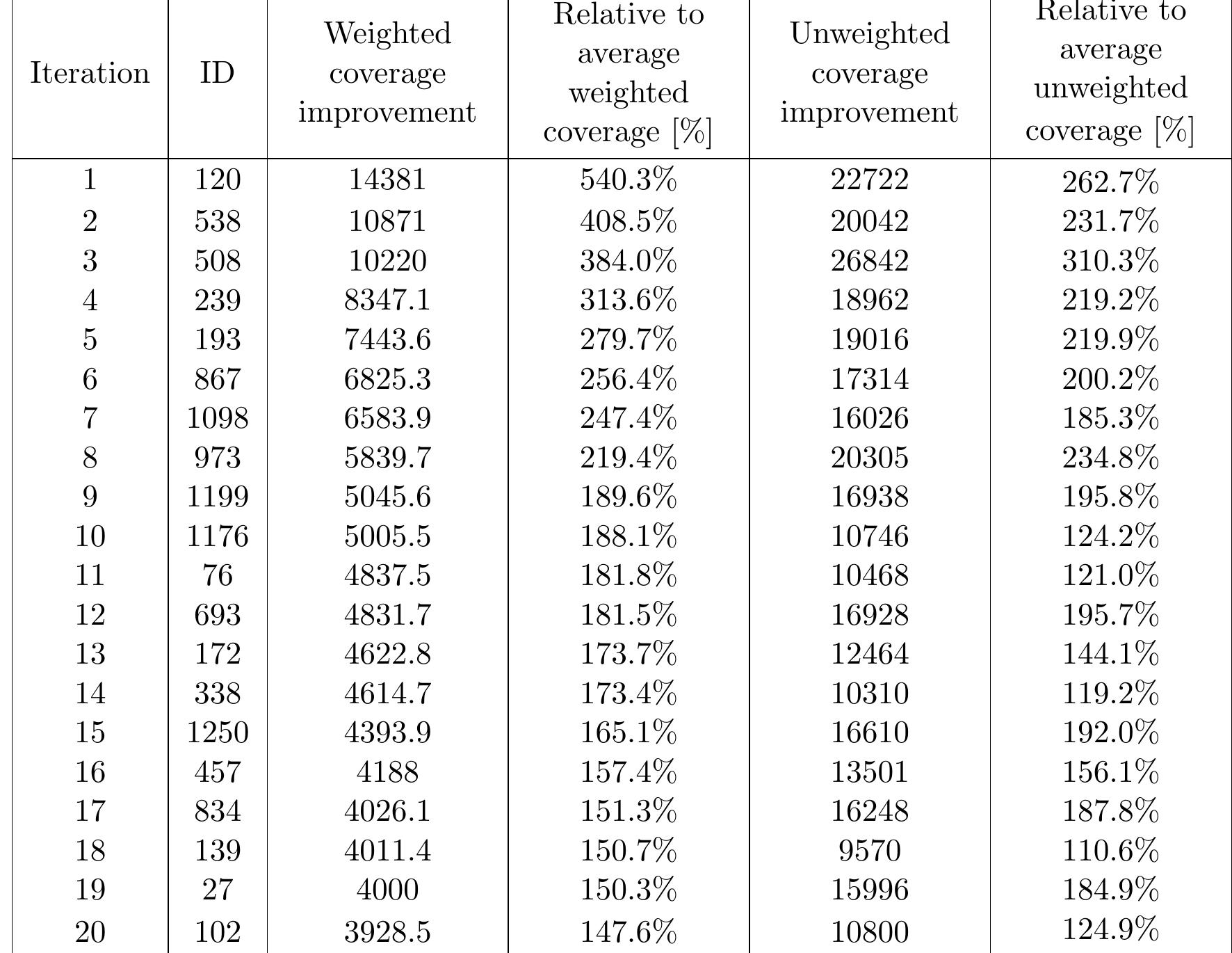
Table 5.1.: Economic Feasibility of supermarket placement: vulnerability-weighted and unweighted coverage from weighted 20-MCLP solution

Loading Preview
Sorry, preview is currently unavailable. You can download the paper by clicking the button above.
References (103)
- American Medical Association (2013). AMA Adopts New Policies on Second Day of Vot- ing at Annual Meeting. URL: http://www.ama-assn.org/ama/pub/news/news/2013/ 2013-06-18-new-ama-policies-annual-meeting.page (accessed January 12, 2014).
- Apparicio, P., M.-S. Cloutier, and R. Shearmur (2007, January). The case of Montréal's missing food deserts: evaluation of accessibility to food supermarkets. International Journal of Health Geographics 6, 1-13.
- Arentze, T., H. Oppewal, and H. Timmermans (2005). A multipurpose shopping trip model to assess retail agglomeration effects. Journal of Marketing Research 42 (1), 109-115.
- Austin, G. L., L. G. Ogden, and J. O. Hill (2011). Trends in carbohydrate, fat, and protein intakes and association with energy intake in normal-weight, overweight, and obese individuals: 1971-2006. The American Journal of Clinical Nutrition 93, 836-843.
- Beasley, J. (1993). Lagrangean heuristics for location problems. European Journal of Operational Research 65, 383-399.
- Beaulac, J., E. Kristjansson, and S. Cummins (2009). A systematic review of food deserts, 1966-2007. Preventing Chronic Disease 6, A105.
- Bell, J., G. Mora, E. Hagan, V. Rubin, and A. Karpyn (2013). Access to Healthy Food and Why It Matters: A Review of the Research. Technical report, The Food Trust, Philadelphia.
- Bitler, M. and S. J. Haider (2011, December). An economic view of food deserts in the united states. Journal of Policy Analysis and Management 30 (1), 153-176.
- Brunett, D. and K. Pothukuchi (2002). Supermarket Access in Low-Income Communities. Technical report, Prevention Institute for the Center for Health Improvement, Oakland, CA. Buss, D. (2013). Whole Foods Opens In Detroit, But Don't Get Maudlin Over It. URL: http://www.forbes.com/sites/dalebuss/2013/06/05/ whole-foods-opens-in-detroit-but-dont-get-maudlin-over-it/ (accessed January 20, 2014). Centers for Disease Control and Prevention (2013). BRFSS 2012 Survey Data and Doc- umentation. URL: http://www.cdc.gov/brfss/annual\_data/annual\_2012.html (ac- cessed January 26, 2014).
- Chung, C. and S. L. Myers (1999). Do the Poor Pay More for Food? An Analysis of Grocery Store Availability and Food Price Disparities. Journal of Consumer Affairs 33, 276-296.
- Church, R. and C. ReVelle (1974, January). The maximal covering location problem. Papers in Regional Science 32 (1), 101-118.
- Church, R. L. (2002). Geographical information systems and location science. Computers & Operations Research 29 (6), 541-562.
- Church, R. L. and C. S. ReVelle (2010, September). Theoretical and Computational Links between the p-Median, Location Set-covering, and the Maximal Covering Location Problem. Geographical Analysis 8 (4), 406-415.
- Church, R. L. and P. Sorensen (1994). Integrating Normative Location Models into GIS: Problems and Prospects with the p-median Model. Technical Report 94-5. Technical report, NCGIA, Santa Barbara.
- Clarke, G., H. Eyre, and C. Guy (2002). Deriving indicators of access to food retail provision in British cities: studies of Cardiff, Leeds and Bradford. Urban Studies 39 (11), 2041-2060.
- Cotterill, R. W. and A. W. Franklin (1995). The urban grocery store gap. Technical report, University of Connecticut, Department of Agricultural and Resource Economics, Charles J. Zwick Center for Food and Resource Policy, Storrs, CT.
- Cummins, S. and S. Macintyre (2002). "Food deserts"-evidence and assumption in health policy making. BMJ 325, 436-438.
- Daskin, M. S. (2013, September). Network and Discrete Location: Models, Algorithms, and Applications (Second Edi ed.). Hoboken, New Jersey: John Wiley & Sons, Inc. Department of Health (1996). Low income, food, nutrition and health: strategies for improvement. A Report from the Low Income Project Team to the Nutrition Task Force. Technical report, Department of Health, London.
- Donkin, A. J., E. A. Dowler, S. J. Stevenson, and S. A. Turner (1999, January). Mapping access to food at a local level. British Food Journal 101 (7), 554-564.
- Drezner, Z. and H. W. Hamacher (2002). Facility location: applications and theory. Berlin; Heidelberg; New York: Springer.
- Duane Perry (2001). The Need for More Supermarkets in Philadelphia. Technical report, The Food Trust, Philadelphia.
- Eckert, J. and S. Shetty (2011, October). Food systems, planning and quantifying access: Using GIS to plan for food retail. Applied Geography 31 (4), 1216-1223.
- Eisenhauer, E. (2001, February). In poor health: Supermarket redlining and urban nutri- tion. GeoJournal 53 (2), 125-133.
- Farahani, R. and M. Hekmatfar (2009). Facility location: concepts, models, algorithms and case studies. Berlin Heidelberg: Springer-Verlag.
- FindTheData (2014). SNAP Retailers | Food Stamp Locations. URL: http:// snap-retailers.findthedata.org (accessed February 17, 2014).
- Finkelstein, E., J. Trogdon, J. Cohen, and W. Dietz (2009). Annual medical spending attributable to obesity: payer-and service-specific estimates. Health Affairs 28 (5), 822- 831.
- Fox, E., S. Postrel, and A. McLaughlin (2007). The impact of retail location on retailer revenues: An Empirical investigation. Technical report, Southern Methodist University, Dallas, TX.
- George, D. and P. Mallery (2003). SPSS for Windows step by step: A simple guide and reference. 11.0 update (4th editio ed.), Volume 11.0 updat. Boston: Pearson Education, Inc. Get Healthy Philly (2011). Farmers' Market and Philly Food Bucks 2010 Report. Technical report, Philadelphia Department of Public Health, Philadelphia, PA.
- Get Healthy Philly (2013). Walkable Access to Healthy Food in Philadelphia, 2010-2012. Technical report, Philadelphia Department of Public Health, Philadelphia, PA.
- Giang, T., A. Karpyn, H. B. Laurison, A. Hillier, and R. D. Perry (2008). Closing the grocery gap in underserved communities: the creation of the Pennsylvania Fresh Food Financing Initiative. Journal of Public Health Management Practice 14 (3), 272-279.
- Gilewicz, N. (2011). Zoning. URL: http://www.nextgreatcity.com/taxonomy/term/14 (accessed January 26, 2014).
- Glanz, K., J. F. Sallis, B. E. Saelens, and L. D. Frank (2007). Nutrition Environment Measures Survey in stores (NEMS-S): development and evaluation. American Journal of Preventive Medicine 32, 282-289.
- Google Developers (2014). The Google Directions API -Google Maps API Web Services. URL: https://developers.google.com/maps/documentation/directions (accessed February 27, 2014).
- Hendrickson, D., C. Smith, and N. Eikenberry (2006). Fruit and vegetable access in four low-income food deserts communities in Minnesota. Agriculture and Human Values 23, 371-383.
- Hillier, A., C. C. Cannuscio, A. Karpyn, J. McLaughlin, M. Chilton, and K. Glanz (2011). How Far Do Low-Income Parents Travel to Shop for Food? Empirical Evidence from Two Urban Neighborhoods. Urban Geography 32, 712-729.
- Hotelling, H. (1929). Stability in competition. The Economic Journal 39, 41-57.
- Jackson, K. (1985). Crabgrass frontier: The suburbanization of the United States. New York: Oxford University Press.
- Karasakal, O. and E. K. Karasakal (2004). A maximal covering location model in the presence of partial coverage. Computers & Operations Research 31 (9), 1515-1526.
- Kaufman, P. R., J. M. MacDonald, S. M. Lutz, and D. M. Smallwood (1997). Do the Poor Pay More for Food? Item Selection and Price Differences Affect Low-Income Household Food Costs. Technical report, Food and Rural Economics Division, Economic Research Service, U.S. Department of Agriculture.
- Kimberly, L. (2011). Get Healthy Philly: Policy Change to Promote Healthy Eating, Active Living, and Tobacco Control. Population Health Matters (Formerly Health Policy Newsletter) 24 (1), 1.
- Kwan, M.-P., A. T. Murray, M. E. O'Kelly, and M. Tiefelsdorf (2003, May). Recent ad- vances in accessibility research: Representation, methodology and applications. Journal of Geographical Systems 5 (1), 129-138.
- Laerd Statistics (2014). How to perform a principal components analysis (PCA) in SPSS. URL: https://statistics.laerd.com/spss-tutorials/ principal-components-analysis-pca-using-spss-statistics.php (accessed February 10, 2014).
- Larsen, K. and J. Gilliland (2008). Mapping the evolution of 'food deserts' in a Canadian city: supermarket accessibility in London, Ontario, 1961-2005. International Journal of Health Geographics 7, 16.
- Leete, L., N. Bania, and A. Sparks-Ibanga (2012). Congruence and Coverage: Alterna- tive Approaches to Identifying Urban Food Deserts and Food Hinterlands. Journal of Planning Education and Research 32, 204-218.
- Levi, J., L. M. Segal, R. S. Laurent, and D. Kohn (2011). F as in Fat : How obesity threatens America's future. Technical report, Trust for America's Health, Washington, DC.
- Lewis, L. B., D. C. Sloane, L. M. Nascimento, A. L. Diamant, J. J. Guinyard, A. K. Yancey, and G. Flynn (2005). African Americans' access to healthy food options in South Los Angeles restaurants. American Journal of Public Health 95, 668-673.
- Longley, P. A., M. F. Goodchild, D. J. Maguire, and D. W. Rhind (1999). Geographical information systems: principles, techniques, applications and management (2nd unabri ed.). New York: John Wiley & Sons, Inc.
- Lopez, R. P. (2007). Neighborhood risk factors for obesity. Obesity 15, 2111-2119.
- Manchikanti, L., D. L. Caraway, A. T. Parr, B. Fellows, and J. a. Hirsch (2011). Patient Protection and Affordable Care Act of 2010: reforming the health care reform for the new decade. Pain Physician 14, E35-67.
- Mantovani, R. E. (1997). Authorized Food Retailer Characteristics Study: Technical Report IV : Authorized Food Retailers' Characteristics and Access Study. Technical report, U.S. Dept. of Agriculture, Food and Consumer Service, Office of Analysis and Evaluation, Alexandria, VA.
- Maranzana, F. (1964). On the location of supply points to minimize transport costs. OR 15 (3), 261-270.
- Maslow, A. H. (1943). A theory of human motivation. Psychological Review 50 (4), 370- 396.
- McEntee, J. and J. Agyeman (2010, January). Towards the development of a GIS method for identifying rural food deserts: Geographic access in Vermont, USA. Applied Geog- raphy 30 (1), 165-176.
- Mieszkowski, P. and E. Mills (1993). The causes of metropolitan suburbanization. The Journal of Economic Perspectives 7 (3), 135-147.
- Miller, H. J. (1996). GIS and geometric representation in facility location problems. Geo- graphical Information Systems 10 (7), 791-816.
- Morland, K., A. V. Diez Roux, and S. Wing (2006). Supermarkets, Other Food Stores, and Obesity. American Journal of Preventive Medicine 30 (4), 333-339.
- Munshi, N. (2013). Whole Foods targets low-income market in Chicago's mean streets. URL: http://www.ft.com/intl/cms/s/0/ 1c3375e6-1b36-11e3-b781-00144feab7de.html (accessed January 20, 2014).
- Murray, A. T., M. E. O. Kelly, and R. L. Church (2008). Regional service coverage modeling. Computers & Operations Research 35, 339-355.
- Office Of The Surgeon General (2001). The Surgeon General's Call to Action To Prevent and Decrease Overweight and Obesity: Overweight in Children and Adolescents. Health San Francisco 2007, 1-39.
- Ogden, C. L., M. D. Carroll, B. K. Kit, and K. M. Flegal (2012). Prevalence of obesity in the United States, 2009-2010. Technical report, National Center for Health Statistics, Hyattsville, MD.
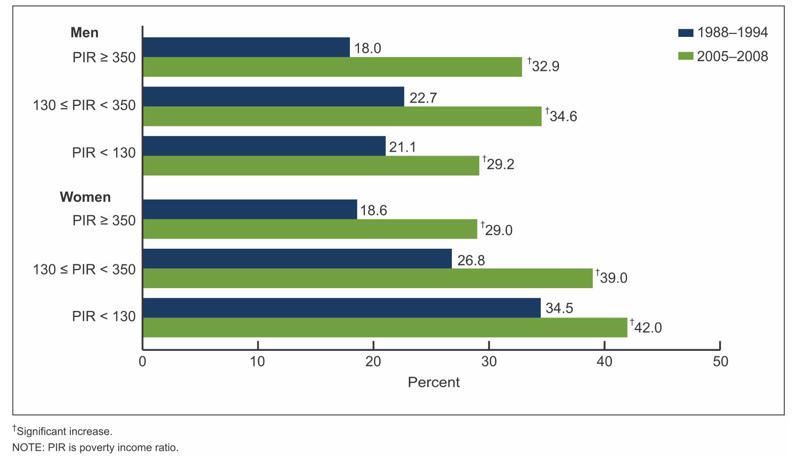
- Ogden, C. L., M. M. Lamb, M. D. Carroll, and K. M. Flegal (2010). Obesity and socioe- conomic status in adults: United States, 2005-2008. Technical report, National Center for Health Statistics, Hyattsville, MD.
- Open Data Philly (2012). Healthy Corner Store Locations. URL: http://www. opendataphilly.org/opendata/resource/216/healthy-corner-store-locations/ (accessed January 28, 2014).
- Open Data Philly (2013). Farmers Markets Locations. URL: http://www. opendataphilly.org/opendata/resource/217/farmers-markets-locations/ (accessed January 28, 2014).
- Owen, S. H. and M. S. Daskin (1998, December). Strategic facility location: A review. European Journal of Operational Research 111 (3), 423-447.
- Ploeg, M. V., V. Breneman, T. Farrigan, K. Hamrick, D. Hopkins, P. Kaufman, B.-h. Lin, M. Nord, T. Smith, R. Williams, K. Kinnison, C. Olander, A. Singh, E. Tuckermanty, R. Krantz-kent, C. Polen, H. Mcgowan, and S. Kim (2009). Access to Affordable and Nutritious Food : Measuring and Understanding Food Deserts and Their Consequences Report to Congress. Technical Report June, United States Department of Agriculture.
- Pothukuchi, K. (2005, August). Attracting Supermarkets to Inner-City Neighborhoods: Economic Development Outside the Box. Economic Development Quarterly 19 (3), 232- 244.
- Pothukuchi, K. and J. Kaufman (1999). Placing the food system on the urban agenda: The role of municipal institutions in food systems planning. Agriculture and Human Values 16, 213-224.
- Powell, L. M., S. Slater, D. Mirtcheva, Y. Bao, and F. J. Chaloupka (2007). Food store availability and neighborhood characteristics in the United States. Preventive Medicine 44, 189-195.
- QGIS Development Team (2014). PyQGIS Developer Cookbook. URL: http://www. qgis.org/en/docs/pyqgis_developer_cookbook/intro.html (accessed February 28, 2014).
- ReVelle, C. and H. Eiselt (2005). Location analysis: A synthesis and survey. European Journal of Operational Research 165, 1-19.
- ReVelle, C., D. Marks, and J. C. Liebman (1970, July). An Analysis of Private and Public Sector Location Models. Management Science 16 (11), 692-707.
- Roddenberry, D. and J. Fleming (2013). Do Obamacare wellness incentives penal- ize the poor and overweight? URL: http://ebn.benefitnews.com/blog/ebviews/ do-obamacare-wellness-incentives-penalize-the-poor-and-overweight-2738050-1. html (accessed January 12, 2014).
- Schafft, K. a., E. B. Jensen, and C. C. Hinrichs (2009). Food Deserts and Overweight Schoolchildren: Evidence from Pennsylvania. Rural Sociology 74, 153-177.
- Sharkey, J. R. and S. Horel (2008). Neighborhood socioeconomic deprivation and minority composition are associated with better potential spatial access to the ground-truthed food environment in a large rural area. The Journal of Nutrition 138, 620-627.
- Simon, H. (1972). Theories of Bounded Rationality. In C. B. McGuire and R. Radner (Eds.), Decision and Organization, pp. 161-176. Amsterdam: North-Holland Publishing Company.
- Sparks, A., N. Bania, and L. Leete (2009). Finding Food Deserts: Methodology and Measurement of Food Access in Portland , Oregon. In National Poverty Center/USDA Economic Research Service research conference "Understanding the Economic Concepts and Characteristics of Food Access", Washington, DC, pp. 54. University of Oregon.
- Stiegert, K. W. and T. Sharkey (2007, January). Food pricing, competition, and the emerging supercenter format. Agribusiness 23 (3), 295-312.
- Swinburn, B. A. (2009, April). Commentary: Closing the disparity gaps in obesity. Inter- national Journal of Epidemiology 38 (2), 509-11.
- Swinburn, B. A., I. Caterson, J. C. Seidell, and W. P. T. James (2004). Diet, nutrition and the prevention of excess weight gain and obesity. Public Health nutrition 7, 123-146.
- Teitz, M. B. and P. Bart (1968). Heuristic Methods for Estimating the Generalized Vertex Median of a Weighted Graph. Operations Research 16, 955-961.
- The Food Trust (2012). Philadelphia's Healthy Corner Store Initiative 2010-2012. Tech- nical report, The Food Trust, Philadelphia.
- The Reinvestment Fund (2012). Searching for Markets: The Geography of Inequitable Access to Healthy & Affordable Food in the United States. Technical report, CDFI Fund, Philadelphia, PA.
- Toivanen, O. and M. Waterson (2005). Market Structure and Entry: Where's the Beef? RAND Journal of Economics 36 (3), 680-699.
- Toregas, C., R. Swain, C. ReVelle, and L. Bergman (1971, October). The Location of Emergency Service Facilities. Operations Research 19 (6), 1363-1373.
- United States Census Bureau (2010a). TIGER Products. URL: http://www.census.gov/ geo/maps-data/data/tiger.html (accessed February 8, 2014).
- United States Census Bureau (2010b). TIGER/Line R with Demographic Data. URL: http://www.census.gov/geo/maps-data/data/tiger-data.html (accessed February 8, 2014).
- United States Census Bureau (2013). Population Estimates. URL: http://www.census. gov/popest/data/state/totals/2013/index.html (accessed January 26, 2014).
- United States Census Bureau (2014a). American Community Survey Summary File. URL: http://www.census.gov/acs/www/data\_documentation/summary\_file/ (ac- cessed February 10, 2014).
- United States Census Bureau (2014b). Philadelphia County QuickFacts from the US Census Bureau. URL: http://quickfacts.census.gov/qfd/states/42/42101.html (accessed February 8, 2014).
- United States Department of Agriculture (2014). SNAP Retailer Locator | Food and Nutrition Service. URL: http://www.fns.usda.gov/snap/retailerlocator (accessed February 17, 2014).
- United States Department of Health Agricultural Marketing Service (2013). Farmers Mar- ket Growth. URL: http://www.ams.usda.gov/AMSv1.0/ams.fetchTemplateData. do?template=TemplateS&navID=WholesaleandFarmersMarkets&leftNav= WholesaleandFarmersMarkets&page=WFMFarmersMarketGrowth&description= Farmers%20Market%20Growth&acct=frmrdirmkt (accessed January 28, 2014).
- Urbany, J. E., P. R. Dickson, and A. G. Sawyer (2000). Insights into cross-and within-store price search: retailer estimates vs. consumer self-reports. Journal of Retailing 76 (2), 243-258.
- U.S. Government Printing Office (2008). Food, Conservation, and Energy Act of 2008. URL: http://www.gpo.gov/fdsys/pkg/PLAW-110publ234/pdf/ PLAW-110publ234.pdf (accessed December 27, 2013).
- Vahrenkamp, R. and D. Mattfeld (2007). Logistiknetzwerke: Modelle für Standortwahl und Tourenplanung (1. Auflage ed.). Wiesbaden: Springer Gabler.
- Vyas, S. and L. Kumaranayake (2006, November). Constructing socio-economic status indices: how to use principal components analysis. Health Policy and Planning 21 (6), 459-68.
- Walker, R. E., C. R. Keane, and J. G. Burke (2010). Disparities and access to healthy food in the United States: A review of food deserts literature. Health & Place 16, 876-884.
- Wang, Y. and M. A. Beydoun (2007). The obesity epidemic in the United States-gender, age, socioeconomic, racial/ethnic, and geographic characteristics: a systematic review and meta-regression analysis. Epidemiologic Reviews 29, 6-28.
- Weinberg, Z. (2000). No place to shop: food access lacking in the inner city. Race, Poverty & the Environment 7 (2), 22-24.
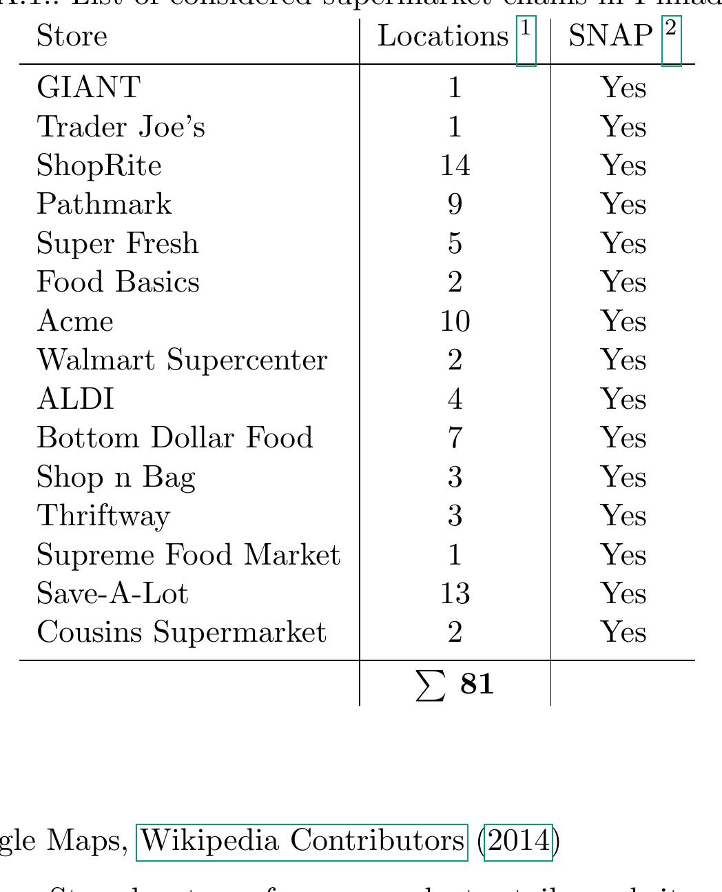
- Wikipedia Contributors (2014). List of supermarket chains in the United States. URL: http://en.wikipedia.org/w/index.php?title=List\_of\_supermarket\_chains\_in\_ the_United_States&oldid=594929611 (accessed February 17, 2014).
- Wolf, A. M. and G. A. Colditz (1998). Current estimates of the economic cost of obesity in the United States. Obesity Research 6, 97-106.
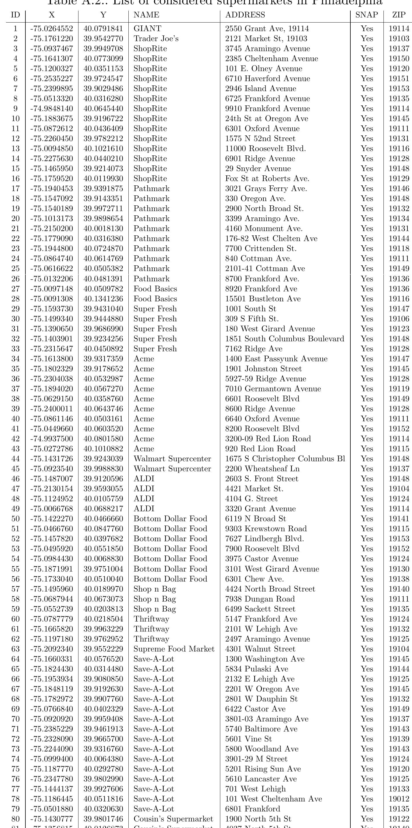
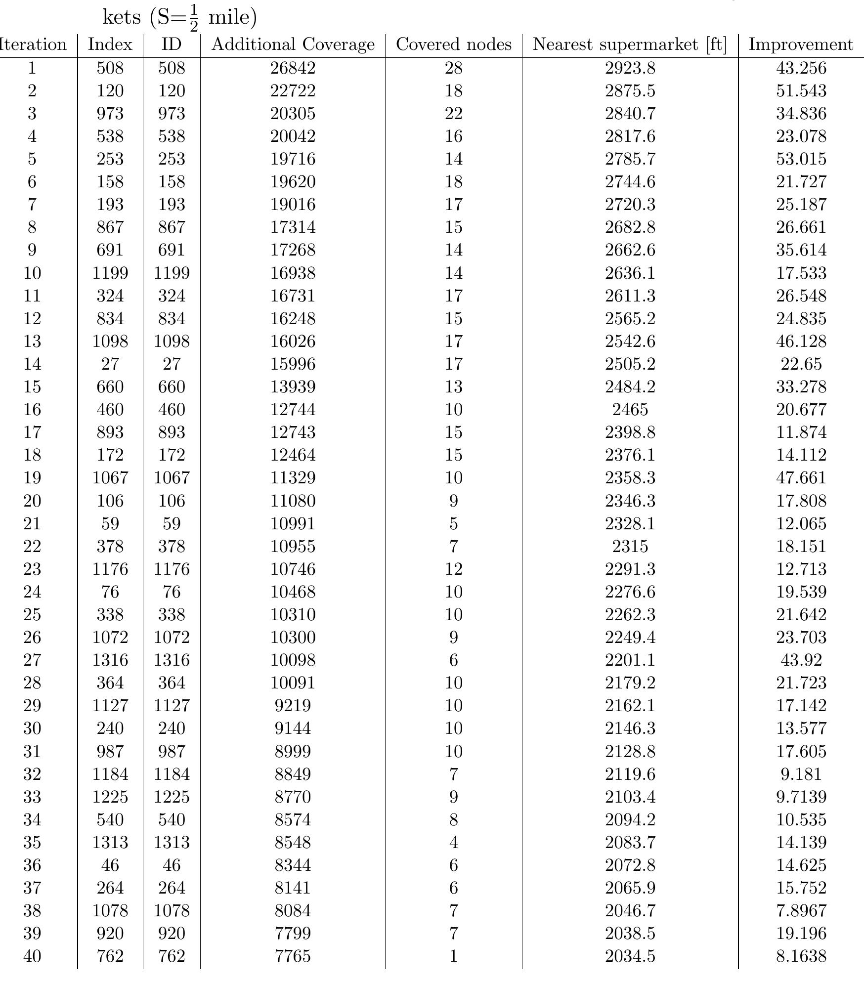
- 1 -75.0264552 40.0791841 GIANT 2550 Grant Ave, 19114 Yes 2 -75.1761220 39.9542770 Trader Joe's 2121 Market St, 19103 Yes 3 -75.0937467 39.9949708 ShopRite 3745 Aramingo Avenue Yes 4 -75.1641307 40.0773099 ShopRite 2385 Cheltenham Avenue Yes 5 -75.1200327 40.0351153 ShopRite 101 E. Olney Avenue Yes 6 -75.2535227 39.9724547 ShopRite 6710 Haverford Avenue Yes 7 -75.2399895 39.9029486 ShopRite 2946 Island Avenue Yes 8 -75.0513320 40.0316280 ShopRite 6725 Frankford Avenue Yes 9 -74.9848140 40.0645440 ShopRite 9910 Frankford Avenue Yes 10 -75.1883675 39.9196722 ShopRite 24th St at Oregon Ave Yes 11 -75.0872612 40.0436409 ShopRite 6301 Oxford Avenue Yes 12 -75.2260450 39.9782212 ShopRite 1575 N 52nd Street Yes 13 -75.0094850 40.1021610 ShopRite 11000 Roosevelt Blvd. Yes 14 -75.2275630 40.0440210 ShopRite 6901 Ridge Avenue Yes 15 -75.1465950 39.9214073 ShopRite 29 Snyder Avenue Yes 16 -75.1759520 40.0119930 ShopRite Fox St at Roberts Ave. Yes 17 -75.1940453 39.9391875 Pathmark 3021 Grays Ferry Ave. Yes 18 -75.1547092 39.9143351 Pathmark 330 Oregon Ave. Yes 19 -75.1540189 39.9972711 Pathmark 2900 North Broad St. Yes 20 -75.1013173 39.9898654 Pathmark 3399 Aramingo Ave. Yes 21 -75.2150200 40.0018130 Pathmark 4160 Monument Ave. Yes 22 -75.1779090 40.0316380 Pathmark 176-82 West Chelten Ave Yes 23 -75.1944800 40.0724870 Pathmark 7700 Crittenden St. Yes 24 -75.0864740 40.0614769 Pathmark 840 Cottman Ave. Yes 25 -75.0616622 40.0505382 Pathmark 2101-41 Cottman Ave Yes 26 -75.0132206 40.0481391 Pathmark 8700 Frankford Ave. Yes 27 -75.0097148 40.0509782 Food Basics 8920 Frankford Ave Yes 28 -75.0091308 40.1341236 Food Basics 15501 Bustleton Ave Yes 29 -75.1593730 39.9431040 Super Fresh 1001 South St Yes 30 -75.1499340 39.9444880 Super Fresh 309 S Fifth St. Yes 31 -75.1390650 39.9686990 Super Fresh 180 West Girard Avenue Yes 32 -75.1403901 39.9234256 Super Fresh 1851 South Columbus Boulevard Yes 33 -75.2315647 40.0450892 Super Fresh 7162 Ridge Ave Yes 34 -75.1613800 39.9317359 Acme 1400 East Passyunk Avenue Yes 35 -75.1802329 39.9178652 Acme 1901 Johnston Street Yes 36 -75.2304038 40.0532987 Acme 5927-59 Ridge Avenue Yes 37 -75.1894020 40.0567270 Acme 7010 Germantown Avenue Yes 38 -75.0629150 40.0358760 Acme 6601 Roosevelt Blvd Yes 39 -75.2400011 40.0643746 Acme 8600 Ridge Avenue Yes 40 -75.0861146 40.0503161 Acme 6640 Oxford Avenue Yes 41 -75.0449660 40.0603520 Acme 8200 Roosevelt Blvd Yes 42 -74.9937500 40.0801580 Acme 3200-09 Red Lion Road Yes 43 -75.0272786 40.1010882 Acme 920 Red Lion Road Yes 44 -75.1431726 39.9243039 Walmart Supercenter 1675 S Christopher Columbus Bl Yes 45 -75.0923540 39.9988830 Walmart Supercenter 2200 Wheatsheaf Ln Yes 46 -75.1487007 39.9120596 ALDI 2603 S. Front Street Yes 47 -75.2130154 39.9593055 ALDI 4421 Market St. Yes 48 -75.1124952 40.0105759 ALDI 4104 G. Street Yes 49 -75.0066768 40.0688217 ALDI 3320 Grant Avenue Yes 50 -75.1422270 40.0466660 Bottom Dollar Food 6119 N Broad St Yes 51 -75.0466760 40.0847760 Bottom Dollar Food 9303 Krewstown Road Yes 52 -75.1457820 40.0397682 Bottom Dollar Food 7627 Lindbergh Blvd. Yes 53 -75.0495920 40.0551850 Bottom Dollar Food 7900 Roosevelt Blvd Yes 54 -75.0984430 40.0068830 Bottom Dollar Food 3975 Castor Avenue Yes 55 -75.1871991 39.9751004 Bottom Dollar Food 3101 West Girard Avenue Yes 56 -75.1733040 40.0510040 Bottom Dollar Food 6301 Chew Ave. Yes 57 -75.1495960 40.0189970 Shop n Bag 4424 North Broad Street Yes 58 -75.0687944 40.0673073 Shop n Bag 7938 Dungan Road Yes 59 -75.0552739 40.0203813 Shop n Bag 6499 Sackett Street Yes 60 -75.0787779 40.0218504 Thriftway 5147 Frankford Ave Yes 61 -75.1665820 39.9963229 Thriftway 2101 W Lehigh Ave Yes 62 -75.1197180 39.9762952 Thriftway 2497 Aramingo Avenue Yes 63 -75.2092340 39.9552229 Supreme Food Market 4301 Walnut Street Yes 64 -75.1660331 40.0576520 Save-A-Lot 1300 Washington Ave Yes 65 -75.1824430 40.0314480 Save-A-Lot 5834 Pulaski Ave Yes 66 -75.1953934 39.9080850 Save-A-Lot 2132 E Lehigh Ave Yes 67 -75.1848119 39.9192630 Save-A-Lot 2201 W Oregon Ave Yes 68 -75.1782972 39.9907760 Save-A-Lot 2801 W Dauphin St Yes 69 -75.0766840 40.0402329 Save-A-Lot 6422 Castor Ave Yes 70 -75.0920920 39.9959408 Save-A-Lot 3801-03 Aramingo Ave Yes 71 -75.2385229 39.9461913 Save-A-Lot 5740 Baltimore Ave Yes 72 -75.2328090 39.9665700 Save-A-Lot 5601 Vine St Yes 73 -75.2244090 39.9316760 Save-A-Lot 5800 Woodland Ave Yes 74 -75.0999400 40.0064380 Save-A-Lot 3901-29 M Street Yes 75 -75.1187770 40.0292780 Save-A-Lot 5201 Rising Sun Ave Yes 76 -75.2347780 39.9802990 Save-A-Lot 5610 Lancaster Ave Yes 77 -75.1444137 39.9927606 Save-A-Lot 701 West Lehigh Yes 78 -75.1186445 40.0511816 Save-A-Lot 101 West Cheltenham Ave Yes 79 -75.0501880 40.0320630 Save-A-Lot 6801 Frankford Yes 80 -75.1430777 39.9801746 Cousin's Supermarket 1900 North 5th St Yes 81 -75.1356815 40.0126873 Cousin's Supermarket 4037 North 5th St Yes Table B.3.: MCLP solution -placement: Supermarkets, p=40, initial coverage: supermar- kets (S= 1 2 mile) Iteration Index ID Additional Coverage Covered nodes Nearest supermarket [ft] Improvement 1 508 508 26842 28 2923.8 43.256 2 120 120 22722 18 2875.5 51.543 3 973 973 20305 22 2840.7 34.836 4 538 538 20042 16 2817.6 23.078 5 253 253 19716 14 2785.7 53.015 6 158 158 19620 18 2744.6 21.727 7 193 193 19016 17 2720.3 25.187 8 867 867 17314 15 2682.8 26.661
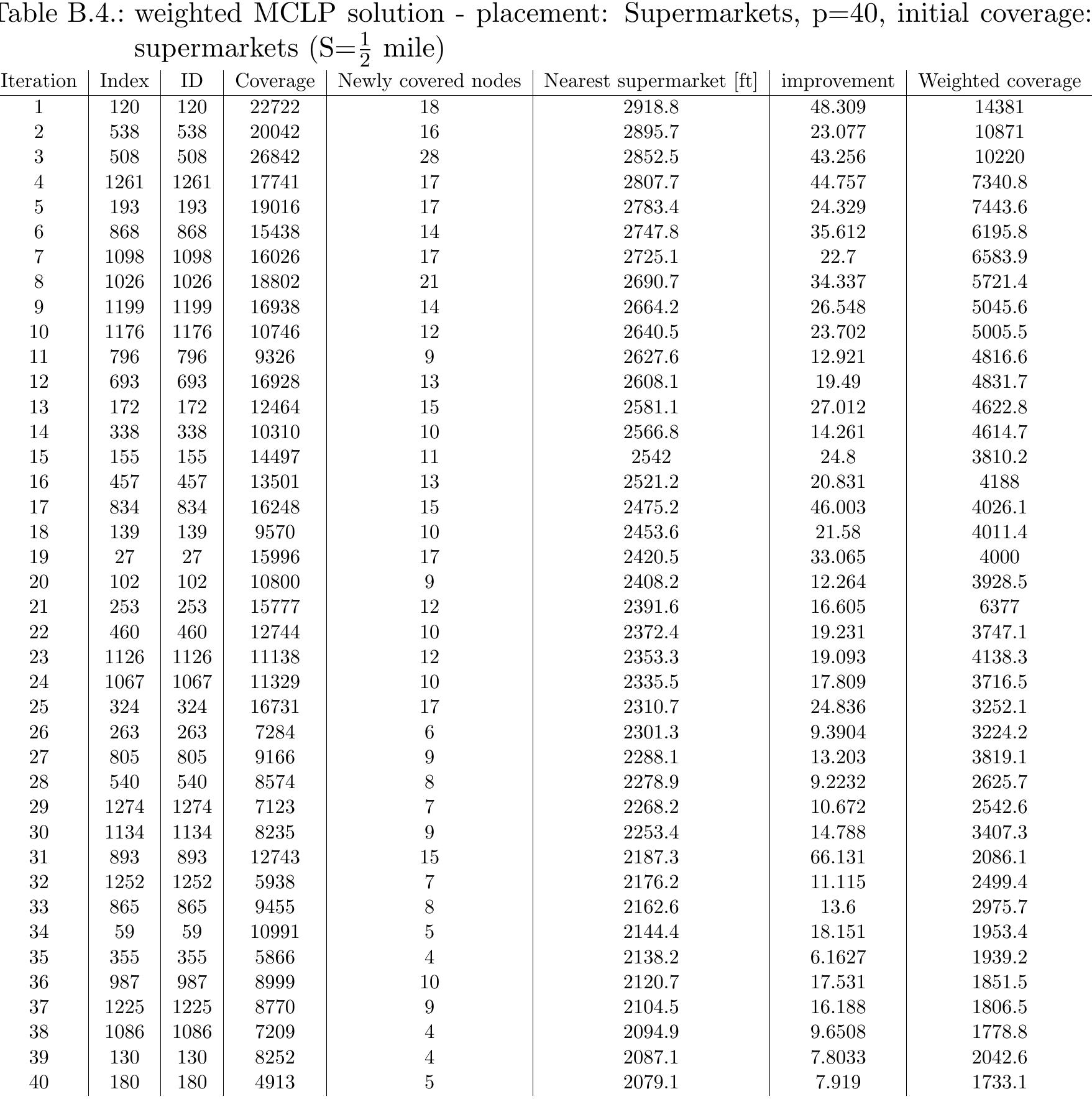
- Table B.4.: weighted MCLP solution -placement: Supermarkets, p=40, initial coverage: supermarkets (S= 1 2 mile) Iteration Index ID Coverage Newly covered nodes Nearest supermarket [ft] improvement Weighted coverage 1 120 120 22722 18 2918.8 48.309 14381 2 538 538 20042 16 2895.7 23.077 10871 3 508 508 26842 28 2852.5 43.256 10220 4 1261 1261 17741 17 2807.7
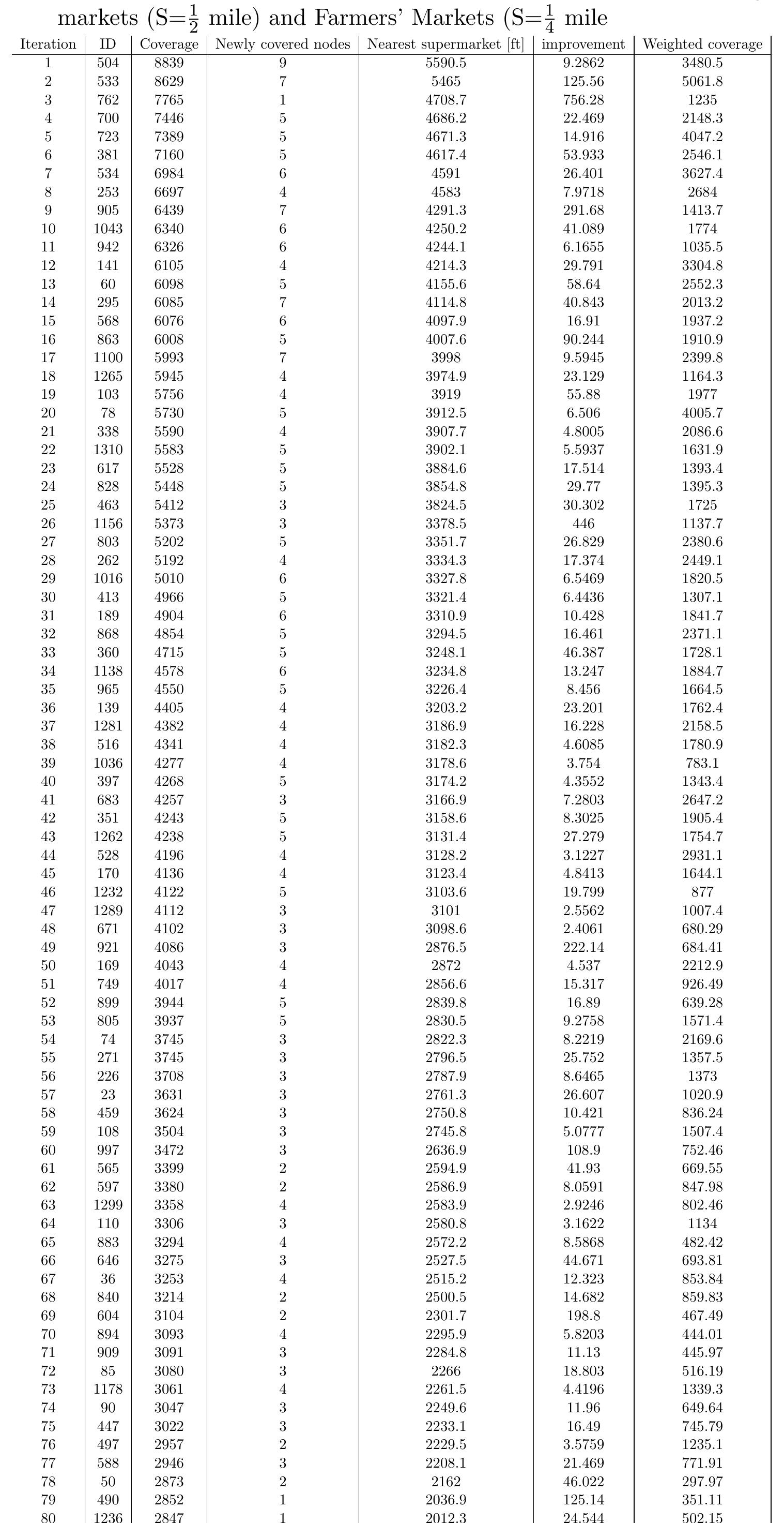
- Table B.5.: MCLP solution -placement: Farmers' Markets, p=80, initial coverage: super- markets (S= 1 2 mile) and Farmers' Markets (S= 1 4 mile Iteration ID Coverage Newly covered nodes Nearest supermarket [ft] improvement Weighted coverage 1 504 8839 9 5590.5