Major Obstacles in Production from Hydraulically Re-fractured Shale Formations: Reservoir Pressure Depletion and Pore Blockage by the Fracturing Fluid (original) (raw)
UNCØNVENTIØNAL
RESOURCES TECHNOLOGY CONFERENCE FUELED BY SPE ⋅\cdot AXIPO ⋅\cdot SEG
URTeC: 2154393
Major Obstacles in Production from Hydraulically Re-fractured Shale Formations: Reservoir Pressure Depletion and Pore Blockage by the Fracturing Fluid
Mahdi Haddad*, SPE, Alireza Sanaei, SPE, Emad Waleed Al-Shalabi, SPE, Kamy Sepehrnoori, SPE, The University of Texas at Austin.
Copyright 2015, Unconventional Resources Technology Conference (URTeC) DOI 10.15530/urtec-2015-2154393
This paper was prepared for presentation at the Unconventional Resources Technology Conference held in San Antonio, Texas, USA, 20-22 July 2015.
The URTeC Technical Program Committee accepted this presentation on the basis of information contained in an abstract submitted by the author(s). The contents of this paper have not been reviewed by URTeC and URTeC does not warrant the accuracy, reliability, or timeliness of any information herein. All information is the responsibility of, and, is subject to corrections by the author(s). Any person or entity that relies on any information obtained from this paper does so at their own risk. The information herein does not necessarily reflect any position of URTeC. Any reproduction, distribution, or storage of any part of this paper without the written consent of URTeC is prohibited.
Summary
Gas production from ultra-low permeable shale resources declines drastically at early times upon which organically rich undrained zones are still left at high gas content. In order to enhance nearly flat gas production rates, refracturing virgin zones using the newly emerged technologies has been widely implemented in the past few years. Therefore, numerical optimizing tools for re-fracturing must capture several production steps including the irreversible reservoir conditions; the depleted reservoir pressure and the associated fracturing fluid pore blockage close to hydraulic fractures. These have not been considered in the production models in the literature.
In this paper, we introduce a multi-step production model including intermediate fracturing fluid injection and soaking time, followed by a detailed sensitivity analysis for the most influential parameters in gas production. A synthetic shale gas reservoir model is created with logarithmically spaced, locally refined grids (LS-LR) inside the stimulated reservoir volume to accurately capture the physics of flow in shale gas reservoirs. This model consists of the following sequential steps: 1) production from the first set of hydraulic fractures and well shut-in at the refracturing time; 2) activation of the second set of hydraulic fractures induced by re-fracturing, and fracturing fluid (water) injection into all fractures to simulate the fracturing fluid invasion into the matrix; 3) fracturing fluid soaking period; and 4) production from the renovated fracture network (the new and old hydraulic fractures). This model provides a mechanistic approach to include and simulate the following obstacles in gas production enhancement using re-fracturing: 1) reservoir pressure depletion in the initially stimulated reservoir volume as the depleted reservoir pressure cannot strongly repel the invaded fracturing fluid out of the matrix; 2) deep fracturing fluid invasion due to the pressure depletion and the alteration of single phase flow to two phase flow.
The results showed that the pressure depletion and the resultant water retainment in the pore space reduced the production enhancement by 5%5 \% compared to the base case without these effects. This modification in gas production can influence the risk assessments for further investment on re-fracturing a field yet producing at low rates, and may revise the number of considered fields for re-fracturing.
Introduction
Shale gas resources have profoundly contributed to the long-term independence of the US on oil and gas from foreign resources. According to EIA (2013), the abundance of these organic-rich formations all over the US can shift the US from a gas importer to an exporter by 2019 only in case the production from these reserves is exploited using the modern technologies of horizontal drilling and hydraulic fracturing. These technologies enhance the reservoir drainage area by providing complex networks of flow channels and activating gas desorption that is one of the major producing mechanisms from shale resources. In practice, these technologies have substantially proliferated gas production, for instance, three orders of magnitude in Woodford Shale during six years (French et al. 2014).
Shale plays are commonly characterized by their ultra-low permeability in the order of nano-Darcies, which demonstrates the resistance of the shale matrix to gas production. Therefore, shale plays are completed by closely spaced fractures presumably with optimal fracture spacing. Nevertheless, the abrupt gas production decline during the first few decades raises several concerns including optimizing initial fracture spacing, re-fracturing treatment to enhance production, and selection of optimal re-fracturing time (Tavassoli et al. 2013). The investigation of optimal fracture spacing requires rigorous fracture mechanics models with the capabilities to include stress interactions of closely spaced fractures (Haddad and Sepehrnoori 2014a,b and 2015a,b). Due to the recent emergence of economic gas production from shales, the fracture mechanics models for closely spaced hydraulic fracturing is still being revised. These models require substantial development, and intensive CPU and operator times, which discourages reservoir engineers from systematically studying this problem. Without a comprehensive geomechanics reservoir model, the general tendency is toward higher and non-optimum fracture spacing in order to minimize stress interactions or shadowing effect of fractures. Thereby, assuming that the initial fracture spacing was higher than optimal, placing the second set of fractures in between can remedy the sharp primary production decline. Furthermore, acid re-fracturing the primary fracture network or in the new clusters may keep the hydraulic fractures open by etching the fracture walls and creating wormholes in leak-off directions (Pournik et al. 2009); the fracturing fluid leak-off is intuitively enhanced by lower reservoir pressures due to primary production. Moreover, the fracturing fluid penetration and flow-back to and from the shale rocks are governed by various phenomena such as capillary saturation/activation, Fick’s law, and gas desorption (Hayatdavoudi et al. 2015).
Nevertheless, placement of the second set of hydraulic fractures in a depleted reservoir has a commonly underestimated detrimental consequence on ensuing production; the fracturing fluid permeates more into the matrix during the injection process and less out of the matrix during the flow-back. The reason behind the latter is that the pore pressure in the depleted reservoir is less than the virgin reservoir’s pore pressure. Consequently, the secondary long-term gas production is governed by a two-phase flow regime in which the liquid phase is almost immobile in the matrix due to the irreducible water saturation and the hysteresis effect after imbibition (water injection) and drainage (water production) processes in shale rocks (Sigal 2013). This immobile water trapped in the matrix can reduce gas relative permeability as much as one order of magnitude.
Therefore, it is essential in evaluating the effectiveness of the re-fracturing treatment to integrate an intermediate fracturing fluid (water) injection period right before the re-fracturing process while running numerical simulations for the whole operation. This intermediate step of water injection is the main theme of the current work, which is integrated in our numerical simulations for a more reliable and rigorous production estimate. Moreover, this work can result in a more trustworthy economic analysis on the profitability of the re-fracturing process. Furthermore, we conduct a comprehensive sensitivity study on the most significant parameters on gas production using re-fracturing treatment on shale gas reservoirs.
Methodology
Overall, four main steps are followed in our simulations: 1) primary production from a primary set of hydraulic fractures while the secondary hydraulic fractures exist but are not activated in the model; 2) activation of secondary hydraulic fractures through fracture connection to the wellbore, and water injection in all hydraulic fractures during re-fracturing treatment; 3) water soaking (shut-in) period for a short time interval, e.g. a month; and 4) opening both primary and secondary hydraulic fractures to the wellbore and producing from all of them. We presume that refracturing is performed by default after 10 years of production from the primary fractures. Step 2 is accomplished in the model by two virtual injection wells, I1 and I2, coincident with the producing wells, P1 and P2, in order to maintain the wells type in the model all along the simulation. Moreover, the duration of step 3 is based on the common practice in completing the horizontal wellbores in shale resources as the secondary production is not initiated right after re-fracturing and the operators use this period of time for reservoir data acquisition.
Table 1 lists the above mentioned steps and their default durations. By default, primary production starts at 2010 and ends at 2020, and followed by a secondary production starting at 2020 and ending at 2040. A sensitivity study is performed to determine the suitable time period for each of these four steps. For instance, fracturing fluid (water) injection period is investigated for the range of 0.5 to 1.5 days and secondary production for 25 to 35 years. The default values in the table represent the base case and the time ranges are based on typical values in the literature and common field practice. Notably, the duration of Step 4 is a function of primary production interval and not an independent variable as we restrict the overall production period to 40 years.
Table 1: The four steps included in the analysis with their range of investigation
| Step Number | Step Name | Time Duration (default values) | Time Range (for Sensitivity Study) |
|---|---|---|---|
| 1 | Primary production: Opening primary HF to wellbores | 10 years | [5,15][5,15] years |
| 2 | Fracturing fluid (water) injection in all hydraulic fractures | 1 day | [0.5,1.5][0.5,1.5] days |
| 3 | Water soaking (shut-in) period | 1 month | [1,3][1,3] months |
| 4 | Secondary production: Opening all HF to wellbores | 20 years | [25,35][25,35] years |
We assume that the second set of hydraulic fractures propagate similar to the first set; the new fractures propagate perpendicular to the wellbore and have similar properties to the primary fractures. This assumption is reasonable when stress interactions between hydraulic fractures are negligible. These stress interactions are also known as stress shadowing effect, which diminish at higher fracture spacing and can be rigorously investigated using quasi-static fully coupled pore pressure-stress analyses for planar fractures such as the works conducted by Haddad and Sepehrnoori (2014a,b and 2015a,b). Nevertheless, this stress analysis is out of the scope of this study as we assume that the fractures are far enough with a negligible stress showing effect.
The main theme of the current work is to investigate the effect of pressure depletion on re-fracturing water leak-off into the formation and its substantial effect on the secondary production from the re-stimulated reservoir volume. This primary pressure depletion depends on the primary production time; the longer the primary production, the larger the drainage area and the lower the pore pressure in the secondary hydraulic fractures’ planes. Moreover, longer water injection results in longer contact between water and shale rock, which promotes more aggressive water leak-off due to capillary imbibition and huge pore pressure gradients on fracture walls. This later effect gets worse when following the common unconventional field practice of delaying production for a few weeks or a month after re-fracturing. Therefore, a comprehensive re-fracturing study has to be accompanied by a sensitivity study on the time lapse for the aforementioned steps. We mainly focus on the durations of the first, second, and third steps (Table 1) since the first step significantly influences the reservoir pressure draw-down, and the second and third steps switch the gas flow regime from almost single-phase to two-phase. The analysis was conducted using CMOST (Version 2013.12) software program developed by CMG, LLC. This program accelerates the sensitivity studies by taking advantage of proxy models to minimize the number of running cases to fully accomplish the sensitivity study for the whole desired range of target variables.
Results and Discussion
The numerical reservoir model that we used for this study is a generic reservoir model with typical values for rock and fluid properties of a shale reservoir and restricted domain of interest embracing two horizontal wellbores with nine hydraulic fracturing stages (Figure 1a). For simplicity, we assumed that the reservoir is isolated from the boundaries and not connected to any aquifer. A maximum permeability of 2 mD was assigned to the fracture volume based on actual fracture conductivity of 3mD−ft3 \mathrm{mD}-\mathrm{ft} and fracture width of 1.5 ft . Furthermore, Figure 1 shows the computational grid and its refinement around the horizontal wellbores. This refinement is preferable to resolve sharp pore pressure gradients perpendicular and very close to the fracture walls due to the ultra-low permeability of shale rocks. One successful strategy for this refinement is known as LS-LR model, which refines the grid logarithmically toward the fracture walls (Figure 1b), and significantly decreases the computational expenses while maintaining the accuracy of the solution (Rubin 2010). Furthermore, we neglected Klinkenberg effect and Knudsen diffusion because these phenomena contribute only in low-pressure flow regimes for the shale pore size distribution, e.g. during shale permeability measurements in laboratory conditions (Sanaei et al. 2014a,b). In order to complete the definition of the model, the relative permeability curves are shown in Figure 2 and Table 2 summarizes the values for geometrical dimensions and properties of the studied reservoir.
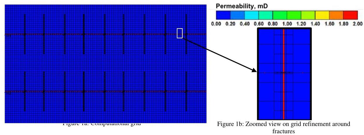
Figure 1: The geometry of reservoir, horizontal wellbores, and hydraulic fractures, and gridding using LS-LR technique (left figure).
Table 2: Properties of investigated shale gas reservoir model
| Parameter | Default value | Unit |
|---|---|---|
| Reservoir dimensions | 2650×1700×502650 \times 1700 \times 50 | ft3\mathrm{ft}^{3} |
| Top horizon depth | 9000 | ft |
| Initial reservoir pore pressure | 5000 | psia |
| Fracture spacing | ∼250\sim 250 | ft |
| Fracture half length | 250 | ft |
| Fracture height | 50 | ft |
| Fracture conductivity | 3 | mD−ft\mathrm{mD}-\mathrm{ft} |
| Number of fracturing stages | 9 stages; 5 primary and 4 secondary stages | 1 |
| Reservoir temperature | 180 | ∘F{ }^{\circ} \mathrm{F} |
| Matrix permeability | 80 | nD |
| Matrix porosity | 0.05 | 1 |
| Bottom hole pressure | 1000 | psia |
| Gas viscosity | 0.018 | cp |
| Water viscosity | 2.2 | cp |
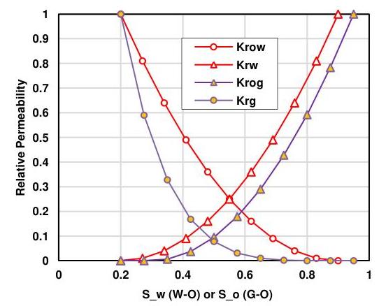
Figure 2: Oil-water and oil-gas relative permeability curves according to a tabulated data set.
Figure 3 shows the pore pressure contours in the reservoir at different times for the default operational parameters in Table 1. Before 2020, the primary hydraulic fractures develop the drainage areas as shown in Figures 3a and 3e as 2D and 3D representations, respectively. These drainage areas can ultimately extend to the planes of the secondary hydraulic fractures, Figure 3b, before secondary hydraulic fracturing. This extension can lead to more water leak-off during the re-fracturing process. Figures 3c, 3d, and 3f demonstrate the development of the drainage areas around all hydraulic fractures after re-fracturing.
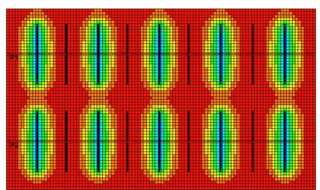
Figure 3a: 2015-1-1, Top view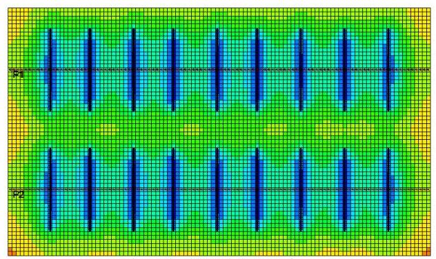
Figure 3c: 2030-1-1, Top view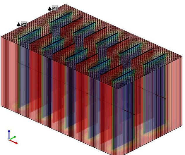
Figure 3e: 2015-1-1, 3D view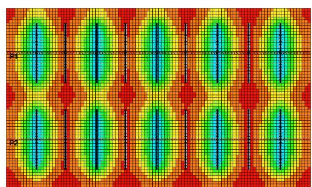
Figure 3b: 2020-2-1, Top view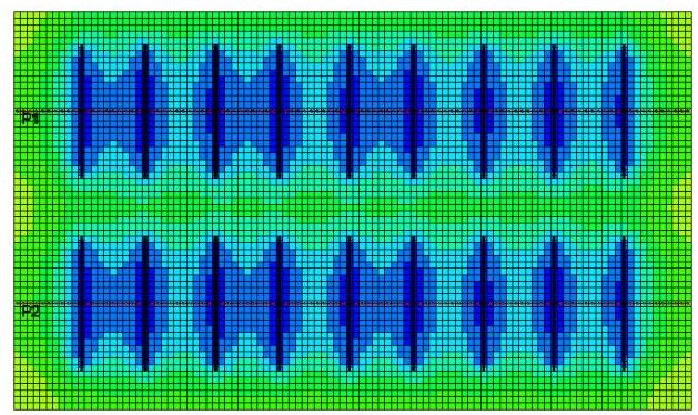
Figure 3d: 2040-1-1, Top view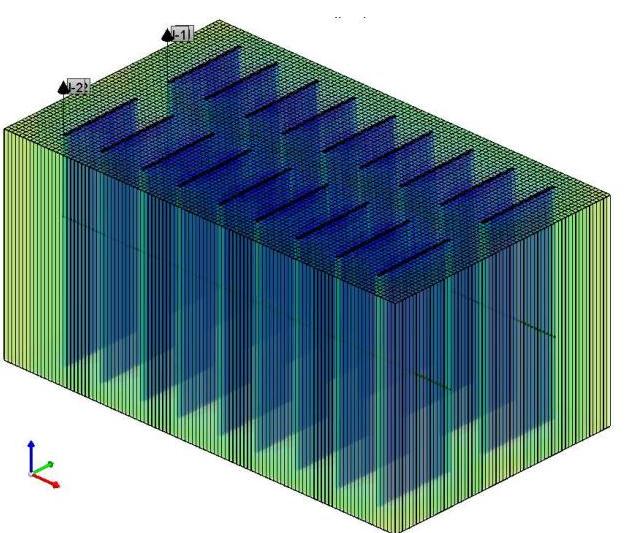
Figure 3f: 2040-1-1, 3D view
1,000 1,400 1,800 2,200 2,600 3,000 3,400 3,800 4,200 4,600 5,000
Figure 3: Pore pressure contours in the reservoir for different dates during production, and before and after re-fracturing for the default valued parameters in Table 1. The pore pressure unit in these contours is psia and the dimension of the model can be found in Table 2.
Figure 4 compares cumulative gas production from Wellbore P1, as shown in Figure 3e, with and without the simulation of the intermediate water injection step during the re-fracturing process. We can observe that the final cumulative gas production in the case with the water injection step is around 20 MMSCF lower than that in the case without water injection step. This significant difference in the cumulative gas production demonstrates the
importance of simulating the intermediate water leak-off during re-fracturing which is neglected in most refracturing simulations.
Figure 5 compares the cumulative water injected for creating the secondary fractures in one horizontal leg and the cumulative produced water during gas production from the same wellbore. The general trend shows the production of half of the water injected after 20 years from the re-fracturing step. This water recovery, 50%50 \%, exceeds the general water recovery of 25%25 \% reported frequently by the hydraulic fracturing operators. This difference can originate from the following: 1) different time scales for these two recovery factors as the operators usually calculate that based on acquired data in short time intervals, e.g. a couple of years, however, our numerical model provides the 50%50 \% recovery factor after 20 years of secondary production; and 2) assumed relative permeability curves for water and gas, which promotes to analyze the sensitivity of the results on the endpoint and exponent values in the Corey’s model for relative permeability in the future work.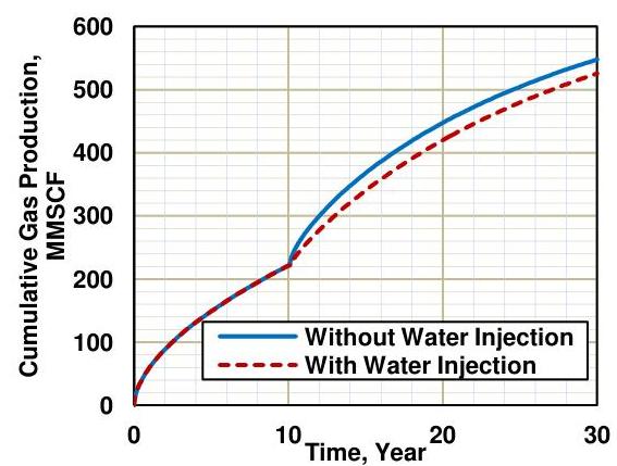
Figure 4: Comparison of cumulative gas production from Wellbore P1 with and without intermediate water injection step, Step 2 in Table 1, which demonstrates the main theme of the current work.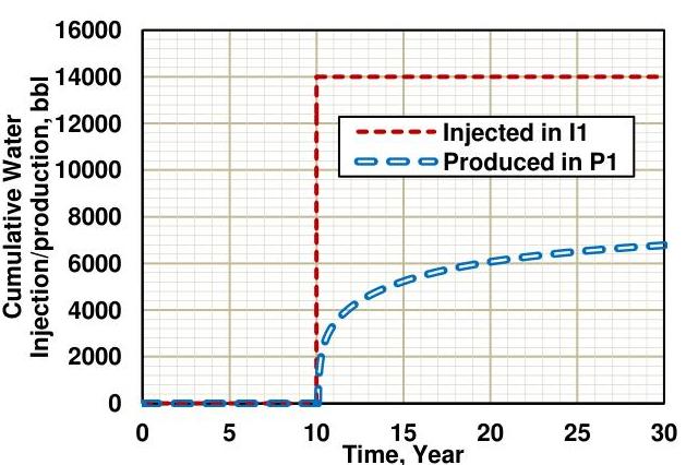
Figure 5: Comparison of injected water in Wellbore I1 during re-fracturing and produced water in Wellbore P1 during gas production.
As the next step, we investigated the time duration effect of the four production steps on both cumulative gas and water productions. This was accomplished using a proxy model in CMOST, response surface methodology. Generally, proxy models require verification as they go through training and verification processes for choosing the combinations of different parameters in the sensitivity study. Therefore, we verified our model by comparing the cumulative gas production and water injection from the simulations with those predicted by the proxy model (Figures 6 and 7). The accumulation of data points on 45-degree line show that the compared values match each other and therefore, the proxy model successfully predicted the simulated cumulative gas production and water injection.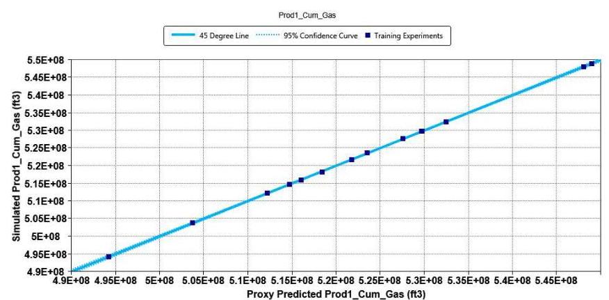
Figure 6: Quality control for the proxy model comparing the simulated and proxy-predicted cumulative gas production from production wellbore P1.
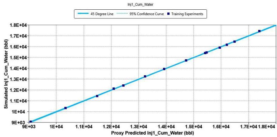
Figure 7: Quality control for the proxy model comparing the simulated and proxy-predicted cumulative injected water in the injection wellbore II.
Having shown that the implemented proxy model can rigorously predict the cumulative gas production and water injection, as the next step, we accomplished a comprehensive sensitivity study on the duration of Steps 1, 2, and 3 listed in Table 1 which correspond to re-fracturing time (primary production period), water injection period, and soaking (shut-in) period after re-fracturing and before secondary production.
Figure 8 shows the effect of changing re-fracturing time (or the number of years for primary production), fracturing fluid (water) injection period during re-fracturing, and post-fracturing shut-in (soaking) period, on the cumulative gas production from one of the production wellbores, P1. The black line represents the base case with default values for different parameters previously listed in Table 1. Also, the blue lines represent the other cases where the values of the parameters in Table 1 were set up according to CMG proxy model and in the assigned range. As observed in this figure, the investigated parameters can change the ultimate gas production by 50 MMSCF at 2050. This variation in gas production majorly originates from variable water invasion in these different cases. Moreover, the maximum cumulative gas production is observed when re-fracturing is conducted after 5 years of production, fracturing fluid is injected only for half a day, and soaking period lasts long for 1 month. In other words, the sooner the re-fracturing, the higher the cumulative gas production. Furthermore, the shorter the water injection and soaking periods, the higher the cumulative gas production.
Figure 9 clearly compares the significance of the investigated parameters in the cumulative gas production in a tornado plot. According to this figure, re-fracturing (or the primary production) time and post-fracturing shut-in (soaking) period have significant effect on the cumulative gas production and the effect of re-fracturing time is higher than soaking period. Obviously, the reservoir drainage area around the primary hydraulic fractures expands more with time and as a result, the later the re-fracturing year, the higher the pressure depletion around the refracturing zones. This can lead to higher fracturing fluid invasion and more pore space blockage due to that, which adversely influences the cumulative gas production afterwards. Our proxy model also provides us with an explicit second order, polynomial equation for the cumulative gas production as a function of the investigated parameters, which can be written as Equation 1.
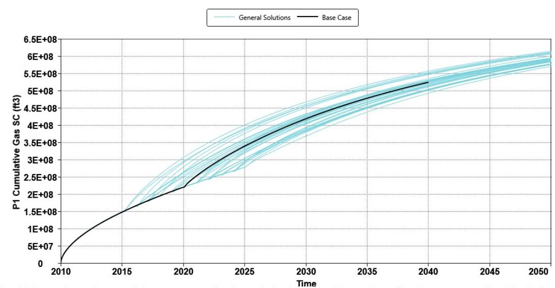
Figure 8: Sensitivity study on the cumulative gas production from the horizontal wellbore P1 varying the parameters listed in Table 1 according to one of the CMOST proxy models, response surface methodology. The middle black line and blue lines correspond to the cumulative gas production for the default and perturbed cases, respectively.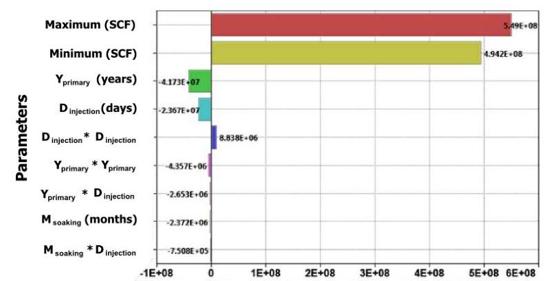
Figure 9: Tornado plot for the investigated parameters affecting the cumulative gas production from wellbore P1. The reduced quadratic proxy model with α=1\alpha=1 was used for this sensitivity study. The higher-order parameters depend on the main three first-order parameters, Yprimary ,Dinjection Y_{\text {primary }}, D_{\text {injection }}, and Msoaking M_{\text {soaking }}.
Cumulative gas production from Wellbore P1:
Qcum,gas, P1=3.48×10¹¹+3.49×10⁸×Yprimary +9.80×10⁸×Dinjection +3.15×10³×Msoaking −8.71×10⁴×Yprimary 2−5.31×10⁵×Yprimary ×Dinjection −7.51×10⁵×Msoaking ×Dinjection +1.77×10⁷×Dinjection 2\begin{aligned} Q_{\text {cum,gas, } P 1}= & 3.48 \times 10^{11}+3.49 \times 10^{8} \times Y_{\text {primary }}+9.80 \times 10^{8} \times D_{\text {injection }}+3.15 \times 10^{3} \times M_{\text {soaking }}-8.71 \times 10^{4} \times Y_{\text {primary }}^{2} \\ & -5.31 \times 10^{5} \times Y_{\text {primary }} \times D_{\text {injection }}-7.51 \times 10^{5} \times M_{\text {soaking }} \times D_{\text {injection }}+1.77 \times 10^{7} \times D_{\text {injection }}^{2} \end{aligned}
where Qcum,gas ,P1,Yprimary ,Dinjection Q_{\text {cum,gas }, P 1}, Y_{\text {primary }}, D_{\text {injection }}, and Msoaking M_{\text {soaking }} denote the cumulative gas production from Well P1 (in SCF), the ending year of primary production, water injection period (in days), and soaking period (in months), respectively. As mentioned before, in this study, the primary production starts at 2010 and lasts for 5 to 15 years, the water injection period varies from 0.5 to 1.5 days, and the soaking period changes from 1 to 3 months.
Furthermore, the cumulative water injection can be stated as a function of the investigated parameters. This functionality is demonstrated in the corresponding tornado plot, Figure 10, and Equation 2. Figure 10 shows that the fracturing fluid (water) injection period causes the highest impact on the cumulative water injection x{ }_{x} and the second influential parameter is the re-fracturing time (or the primary production period). Moreover, according to this tornado plot, the re-fracturing time proportionally affects the cumulative water injection, which again confirms our hypothesis on the significant effect of pressure depletion on the invaded fluid and gas production.
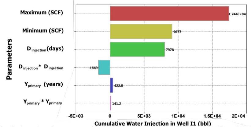
Figure 10: Tornado plot for the investigated parameters affecting the cumulative water injection in wellbore I1. The reduced quadratic proxy model with α=1\alpha=1 was used for this sensitivity study. The higher-order parameters depend on the two first-order parameters, Dinjection D_{\text {injection }} and Yprimary Y_{\text {primary }}.
Cumulative water injection in Wellbore I1:
Qcum, water,inj,II =1.14×10⁷−1.13×10⁴×Yprimary +2.13×10⁴×Dinjection +2.82×Yprimary 2−3.33×10³×Dinjection 2Q_{\text {cum, water,inj,II }}=1.14 \times 10^{7}-1.13 \times 10^{4} \times Y_{\text {primary }}+2.13 \times 10^{4} \times D_{\text {injection }}+2.82 \times Y_{\text {primary }}^{2}-3.33 \times 10^{3} \times D_{\text {injection }}^{2}
where Qcum,water,inj,II Q_{\text {cum,water,inj,II }} denotes the cumulative water (in bbl) injected in Well I1 during re-fracturing, and the independent parameters in the right hand side are defined after Equation 1.
Conclusions
The main findings of this work can be summarized as the following:
- We successfully highlighted the detrimental effect of missing the simulation of intermediate water injection steps on predicted gas production from presented numerical models for the re-fracturing process in the literature.
- The intermediate step was designed and implemented sequentially right after primary gas production from the primary hydraulic fractures: 1) grid modification for the secondary hydraulic fractures; 2) fracturing fluid (water) injection step by defining the injection wellbores similar to the production legs and injecting water in them for a typical time interval for hydraulic fracturing processes; and 3) post-fracturing soaking (shut-in) period according to field practice for data acquisition. We demonstrated the profound effect of water injection during re-fracturing on cumulative gas production by comparing the results with and without water injection and soaking steps.
- The significant effect of considering intermediate water injection step originates from two factors: 1) two-phase gas flow regime very close to the fracture walls after re-fracturing, which leads to more flow resistance to gas phase; 2) pressure depletion around the re-fracturing zones which causes higher fracturing fluid invasion into the matrix. The second factor can aggravate the first one as a bigger invaded volume causes more blockage to the flow of gas toward the hydraulic fractures.
Nomenclature
Yprimary = Ending year of primary production (T), year Dinjection = Fracturing fluid (water) injection period (T), day Msoaking = Fracturing fluid soaking time (T), month Qcum,gas, P1= Cumulative gas production from Well P1 (L3),SCF Qcum,water,inj,II = Cumulative water injected in Well I1 during hydraulic re-fracturing (L3),bbl\begin{aligned} Y_{\text {primary }} & =\text { Ending year of primary production (T), year } \\ D_{\text {injection }} & =\text { Fracturing fluid (water) injection period (T), day } \\ M_{\text {soaking }} & =\text { Fracturing fluid soaking time (T), month } \\ Q_{\text {cum,gas, } P 1} & =\text { Cumulative gas production from Well P1 }\left(\mathrm{L}^{3}\right) \text {,SCF } \\ Q_{\text {cum,water,inj,II }} & =\text { Cumulative water injected in Well I1 during hydraulic re-fracturing }\left(\mathrm{L}^{3}\right), \mathrm{bbl} \end{aligned}
Acknowledgement
We would like to acknowledge the Center for Petroleum and Geosystems Engineering at The University of Texas at Austin for funding this research. Furthermore, we appreciate Computer Modeling Group, LLC for providing academic CMG license to accomplish the current work.
References
CMOST User Manual, Version 2013.12, 2013. Computer Modelling Group (CMG), Calgary, Alberta
Devegowda, D., Sapmanee, K., Civan, F., and Sigal, R.F. 2012. Phase Behavior of Gas Condensates in Shales due to Pore Proximity Effects: Implications for Transport, Reserves and Well Productivity. Paper SPE 160099 presented at the SPE ATCE held in San Antonio, Texas, USA, 8-10 October. http://dx.doi.org/10.2118/160099-MS
EIA, 2013. Annual Energy Outlook, The U.S. Energy Information Administration.
Haddad, M., and Sepehrnoori, K. 2015a. XFEM-Based CZM for the Simulation of 3D Multiple-Stage Hydraulic Fracturing in Quasi-brittle Shale Formations. Presented in the 5th 5^{\text {th }} International Conference on Coupled Thermo-Hydro-Mechanical-Chemical (THMC) Processes in Geosystems: Petroleum and Geothermal Reservoir Geomechanics and Energy Resource Extraction held in Salt Lake City, Utah, USA, 25-27 February.
Haddad, M., and Sepehrnoori, K. 2015b. Simulation of Hydraulic Fracturing in Quasi-brittle Shale Formations Using Characterized Cohesive Layer: Stimulation Controlling Factors. Journal of Unconventional Oil and Gas Resources, 9, 65-83. http://dx.doi.org/10.1016/j.juogr.2014.10.001
Haddad, M., and Sepehrnoori, K. 2014a. Simulation of Multiple-Stage Fracturing in Quasibrittle Shale Formations Using Pore Pressure Cohesive Zone Model. Paper SPE 1922219 presented at the Unconventional Resources Technology Conference held in Denver, Colorado, USA, 25-27 August. http://dx.doi.org/10.15530/urtec-2014-1922219
Haddad, M., and Sepehrnoori, K. 2014b. Cohesive Fracture Analysis to Model Multiple-Stage Fracturing in Quasibrittle Shale Formations. SIMULIA Community Conference, Providence, RI, USA, 19-21 May.
Hayatdavoudi, A., Boamah, M.A., Tavnaei, A., Sawant, K.G., and Boukadi, F. 2015. Post Frac Gas Production through Shale Capillary Activation. Paper SPE 173606-MS presented at the SPE Production and Operations Symposium held in Oklahoma, USA, 1-5 March. http://dx.doi.org/10.2118/173606-MS
French, S., Rodgerson, J., and Feik, C. 2014. Re-fracturing Horizontal Shale Wells: Case History of a Woodford Shale Pilot Project. Paper SPE 168607 presented at the SPE Hydraulic Fracturing Technology Conference held in The Woodlands, Texas, USA, 4-6 February 2014.
Pournik, M., Mahmoud, M., and Nasr-El-Din, H.A. 2009. Acid Re-fracturing: Is it a Good Practice?. Paper SPE 124874 presented at the SPE ATCE held in New Orleans, Louisiana, 4-7 October 2009.
Rubin, B. 2010. Accurate Simulation of Non-Darcy Flow in Stimulated Fractured Shale Reservoirs. Paper SPE 132093 presented at the SPE Western Regional Meeting held in Anaheim, California, USA, 27-29 May 2010.
Sanaei, A., and Jamili, A. 2014a. Optimum Fracture Spacing in the Eagle Ford Gas Condensate Window. Paper SPE 1922964 presented at the Unconventional Resources Technology Conference (URTeC) held in Denver, Colorado, USA, 25-27 August. http://dx.doi.org/10.15530/urtec-2014-1922964
Sanaei, A., Jamili, A., and Callard, J. 2014b. Effects of Non-Darcy Flow and Pore Proximity on Gas Condensate Production from Nanopore Unconventional Resources. Presented in 5th International Conference on Porous Media and Their Applications in Science, Engineering and Industry (ECI Symposium Series) held in Kona, Hawaii, USA, 22-27 June. http://dc.engconfintl.org/ porous_media_V/33
Sigal, R.F. 2013. Mercury Capillary Pressure Measurements on Barnett Core. SPE Reservoir Evaluation & Engineering, 16(4). http://dx.doi.org/10.2118/167607-PA
Tavassoli, S., Yu, W., Javadpour, F., and Sepehrnoori, K. 2013. Well Screen and Optimal Time of Refracturing: A Barnett Shale Well. Journal of Petroleum Engineering, 2013, Article ID 817293. http://dx.doi.org/10.1155/2013/817293