Self-avoiding walks crossing a square (original) (raw)

Abstract

We study a restricted class of self-avoiding walks (SAWs) which start at the origin (0, 0), end at (L, L), and are entirely contained in the square [0, L] × [0, L] on the square lattice Z 2 . The number of distinct walks is known to grow as λ L 2 +o(L 2 ) . We estimate λ = 1.744 550 ± 0.000 005 as well as obtaining strict upper and lower bounds, 1.628 < λ < 1.782. We give exact results for the number of SAWs of length 2L + 2K for K = 0, 1, 2 and asymptotic results for K = o(L 1/3 ). We also consider the model in which a weight or fugacity x is associated with each step of the walk. This gives rise to a canonical model of a phase transition. For x < 1/µ the average length of a SAW grows as L, while for x > 1/µ it grows as L 2 . Here µ is the growth constant of unconstrained SAWs in Z 2 . For x = 1/µ we provide numerical evidence, but no proof, that the average walk length grows as L 4/3 . Another problem we study is that of SAWs, as described above, that pass through the central vertex of the square. We estimate the proportion of such walks as a fraction of the total, and find it to be just below 80% of the total number of SAWs. We also consider Hamiltonian walks under the same restriction. They are known to grow as τ L 2 +o(L 2 ) on the same L × L lattice. We give precise estimates for τ as well as upper and lower bounds, and prove that τ < λ.

Figures (18)

Figure 1. An example of a SAW configuration crossing a square (the left panel), traversing « square from left to right (the middle panel) and a cow-patch (the right panel). anywhere on the left edge of the square and terminate anywhere on the right edge; so these are walks traversing the square from left to right. We call such walks transverse walks. Secondly, we consider the problem in which there may be several independent SAWs, each SAW starting and ending on the perimeter of the square. The SAWs are not allowed to take steps along the edges of the perimeter. Such walks partition the square into distinct regions and by colouring the regions alternately black and white we get a cow-patch pattern. Each problem is illustrated in figure 1.

Table 1. The various ‘input’ states and the ‘output’ states which arise as the boundary line is moved in order to include one more vertex. Each panel contains up to three possible ‘output’ states or other allowed actions.

Figure 2. The left panel shows a snapshot of the intersection (the dashed line) during the transfer matrix calculation. Walks are enumerated by successive moves of the kink in the boundary, as exemplified by the position given by the dotted line, so that the L x M rectangle is built up one vertex at a time. To the left of the boundary we have drawn an example of a partially completed walk. Numbers along the boundary indicate the encoding of this particular configuration. The right panel shows some of the local configurations which occur as the kink in the intersection is moved one step.

Table 2. The total number of walks crossing a square, Cz,(1), cow-patch walks, Pz (1) anc traversing walks, Ty (1).

Figure 3. From transverse walks to walks crossing a square (left). From walks crossing a square to cow-patches (right).

Self-avoiding walks crossing a square

Figure 4. From cow-patches to walks crossing a square.

Figure 5. Dense packings of walks crossing or traversing a square.

Figure 6. A generalized cow-patch.

Figure 7. Enumeration of self-avoiding walks with one vertical defect. 6. Short walks crossing a square

Figure 8. Four types of self-avoiding walks with two defects. The same ideas may be used to find the value of c2744(L). We will prove that

Figure 9. The fluctuations V(x, L) as a function of the fugacity x (the top-left panel). x.(L) — x¢ and Vmax versus L (the top-right panel). V(x, L)/L°/> (the bottom-left panel) and D(x, L) (the bottom-right panel) versus the scaling variable (x — x.) L4/3.

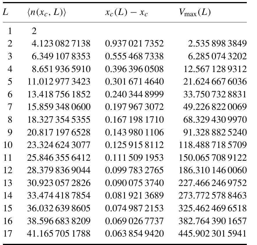
Table 3. The mean-length of walks crossing an L x L square at the critical fugacity x = x;, the position, x-(L) — X¢, and height, Vinax (L), of the peak in the fluctuations V (x, L). Table 4. Estimates for z. and the critical exponents obtained from second-order differential approximants to the generating functions in table 3. K is the degree of the inhomogeneous polynomial of the differential approximant.

the scaling ansatz for V(x, L). In the left panel we plot V(x, L)/L*/> versus the scaling variable (x — x,)L*/* obtaining a reasonable scaling collapse. A better idea of the quality of the scaling collapse can be gauged from the plot in the bottom-right panel. Here we plot the difference between consecutive scaling plots from the left panel. More precisely, we plot D(x, L) = V(x, L)/L8? — V(x’, L—1)/(L — 1)8/? versus (x — x.) L*/?, where x’ is chosen so that the scaled variables coincide, e.g., (x — x.) L477 = (x! — x.)(L — 1)*?.

Table 5. The total number of walks crossing an L x L square and passing through the centre (L/2, L/2), c(L) and the ratio c(L)/C(L). cz) on to say that ’perhaps nobody will ever know the true answer.” Naturally, we cannot let Knuth’s challenge go unanswered. It is very simple to modify the transfer matrix algorithm to ensure that all paths pass through a given vertex. We just make sure that when we do the updating at the given vertex the input state ‘00’ (no occupied incoming edges) has only one output state ‘12’, while the output ‘00’ (no outgoing occupied edges) is disallowed at this vertex. We can thus answer Knuth’s query and state for all to know that for L = 10 a fraction 1243 982 213 040 307 428 318 660/1568 758 030 464 750 013 214 100 = 0.792972... of all paths pass through the centre. In table 5 we have listed the number of paths passing through the centre for L < 18.

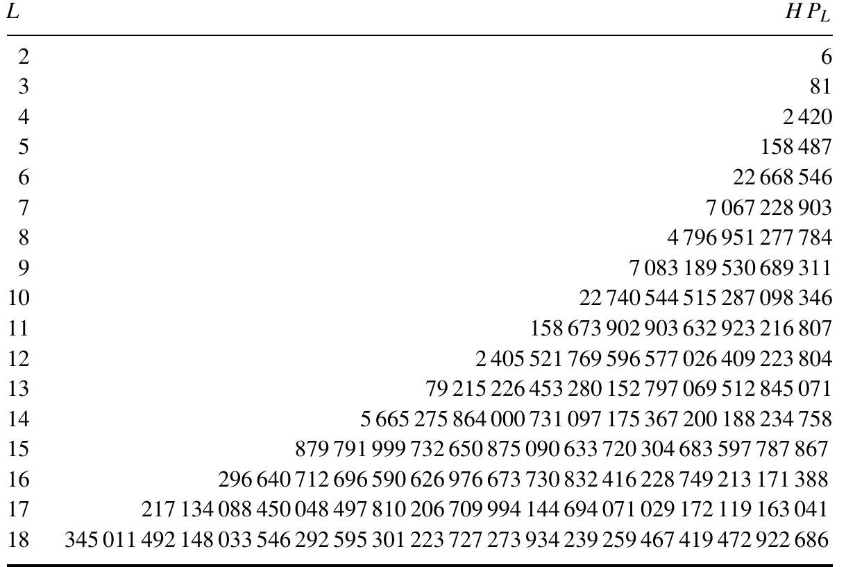
Table 6. The number of Hamiltonian paths. Table 7. The number of Hamiltonian cow-patch paths.

The number of Hamiltonian paths Hz; for L even, and paths that visit all but one site, for L odd, are given in table 6. The number of Hamiltonian cow-patch paths H P; for L even, and cow-patch paths that visit all but one site, for L odd, are given in table 7. The number of Hamiltonian transverse paths HT, for L even, and transverse paths that visit all but one site, for L odd, are given in table 8.

Loading Preview

Sorry, preview is currently unavailable. You can download the paper by clicking the button above.

References (18)

1. Abbott H L and Hanson D 1978 Ars Comb. 6 163
2. Burkhardt T W and Guim I 1991 J. Phys. A: Math. Gen. 24 L1221
3. Cardy J L 1984 Nucl. Phys. B 240 514
4. Collins K L and Krompart L B 1997 Discrete Math. 169 29
5. Conway A R, Enting I G and Guttmann A J 1993 J. Phys. A: Math. Gen. 26 1519
6. Duplantier B and Saleur H 1987 Nucl. Phys. B 290 291
7. Edwards K 1985 Ars Comb. B 20 271
8. Enting I G, Guttmann A J, Richmond L B and Wormald N C 1992 Random Struct. Algorithms 3 445
9. Guttmann A J 1989 Asymptotic analysis of power-series expansions Phase Transitions and Critical Phenomena vol 13, ed C Domb and J L Lebowitz (New York: Academic)
10. Jacobsen J L and Kondev J 1998 Phys. Rev. Lett. 81 2922
11. Knuth D E 1969 Seminumerical Algorithms. The Art of Computer Programming vol 2 (Reading, MA: Addison- Wesley)
12. Knuth D E 1976 Science 194 1235
13. Madras N 1995 J. Phys. A: Math. Gen. 28 1535
14. Madras N and Slade G 1993 The Self-Avoiding Walk (Boston: Birkhäuser)
15. Oxley J G and Welsh D J A 1979 J. Appl. Probab. 16 526
16. Stanley R P 1980 Eur. J. Comb. 1 175
17. Stanley R P 1999 Enumerative Combinatorics Vol 2 (Cambridge Studies in Advanced Mathematics vol 62) (Cambridge: Cambridge University Press)
18. Whittington S G and Guttmann A J 1990 J. Phys. A: Math. Gen. 23 5601